Journal of Biomedical Science and Engineering
Vol.6 No.5(2013), Article ID:31887,10 pages DOI:10.4236/jbise.2013.65070
Random forest classifier combined with feature selection for breast cancer diagnosis and prognostic
![]()
1School of Business and Administration, Chongqing University, Chongqing, China
2College of Technology, Vietnam National University, Hanoi, Vietnam
Email: cuong.ng.vn@gmail.com, *wangyongkt@126.com
Copyright © 2013 Cuong Nguyen et al. This is an open access article distributed under the Creative Commons Attribution License, which permits unrestricted use, distribution, and reproduction in any medium, provided the original work is properly cited.
Received 20 February 2013; revised 4 April 2013; accepted 7 May 2013
Keywords: Breast Cancer; Diagnosis; Prognosis; Feature Selection; Random Forest
ABSTRACT
As the incidence of this disease has increased significantly in the recent years, expert systems and machine learning techniques to this problem have also taken a great attention from many scholars. This study aims at diagnosing and prognosticating breast cancer with a machine learning method based on random forest classifier and feature selection technique. By weighting, keeping useful features and removing redundant features in datasets, the method was obtained to solve diagnosis problems via classifying Wisconsin Breast Cancer Diagnosis Dataset and to solve prognosis problem via classifying Wisconsin Breast Cancer Prognostic Dataset. On these datasets we obtained classification accuracy of 100% in the best case and of around 99.8% on average. This is very promising compared to the previously reported results. This result is for Wisconsin Breast Cancer Dataset but it states that this method can be used confidently for other breast cancer diagnosis problems, too.
1. INTRODUCTION
The high incidence of breast cancer in women has increased significantly in the recent years. It is the cause of the most common cancer death in women (exceeded only by lung cancer) [1]. As reported by WHO, [2] there are about 1.38 million new cases and 458000 deaths from breast cancer each year. Breast cancer is by far the most common cancer both in the developed and developing countries. Breast cancer survival rates vary greatly worldwide, ranging from 80% or over in North America, Sweden and Japan to around 60% in middle-income countries and below 40% in low-income countries.
The use of expert systems and machine learning techniques in medical diagnosis is increasing gradually. There is no doubt that evaluation of data taken from patient and decisions of experts are the most important factors in diagnosis. But, expert systems and different artificial intelligence systems for diagnoses also help experts in a great deal. With the help of automatic diagnostic systems, the possible errors medical experts made in the course of diagnosis can be avoided, and the medical data can be examined in shorter time and more detailed as well.
This study aims to build a computer-aided diagnostic system to distinguish benign breast tumor from malignnant one. This method involves two stages in which a backward elimination approach of feature selection and a learning algorithm random forest are hybridized. The first stage of the whole system conducts a data reduction process for learning algorithm random forest of the second stage. This provides less training data for random forest and so prediction time of the algorithm can be reduced in a great deal. With a selected feature set, the explanation of rationale for the system can be more readily realized.
Our proposed method averagely obtained 99.82% and 99.70% classification accuracy in test phase and these results are the highest one among the studies applied for Wisconsin Breast Cancer Diagnosis Dataset (WBC-DD) and Wisconsin Breast Cancer Prognostic Dataset (WBCPD) classification problem so far. It also indicates that the proposed method can be applied confidently to other breast cancer problems with different data sets especially with ones that have a higher number of training data.
The used data source is Wisconsin Diagnosis Breast Cancer Dataset taken from the University of California at Irvine (UCI) Machine Learning Repository [3]. This data set is commonly used among researchers who use expert systems and machine learning methods for breast cancer diagnosis and so it provides us to compare the performance of our system with other conducted studies related with this problem.
The rest of the paper is organized as follows. Section 2 summarizes the methods and results of previous research on breast cancer diagnosis. Section 3 reviews theoretical background. Section 4 describes the proposed method. Section 5 presents experimental result from using the proposed method to diagnose and prognosis breast cancer. Finally, Section 6 concludes the paper along with outlining future directions.
“Word 97-2003 & 6.0/95-RTF” for the PC, provides authors with most of the formatting specifications needed for preparing electronic versions of their papers. All standard paper components have been specified for three reasons: 1) ease of use when formatting individual papers; 2) automatic compliance to electronic requirements that facilitate the concurrent or later production of electronic products; and 3) conformity of style throughout a journal paper. Margins, column widths, line spacing, and type styles are built-in; examples of the type styles are provided throughout this document and are identified in italic type, within parentheses, following the example. Some components, such as multi-leveled equations, graphics, and tables are not prescribed, although the various table text styles are provided. The formatter will need to create these components, incorporating the applicable criteria that follow.
2. RELATED WORK
There has been a lot of research on medical diagnosis of breast cancer Hui-Ling Chen et al. [4] used a rough set (RS) based supporting vector machine classifier (RS_ SVM) and the reported accuracy was 96.87% in average. Based on neuro-fuzzy rules Ali Keles et al. [5] presented a decision support system for diagnosis breast cancer. As be reported, the system has high positive predictive rate (96%) and specificity (97%). In A. Marcano et al. [6] proposed a method named AMMLP based on the biological meta-plasticity property of neurons and Shannon’s information theory. As reported by authors, the AMMLP obtained total classification accuracy of 99.26%. In Murat Karabatak and M. Cevdet Ince [7] an automatic diagnosis system for detecting breast cancer based on association rules (AR) and neural network (NN) was proposed. The reported correct classification rate of proposed system was at 95.6%. In Kemal Polat and Salih Güne [8] breast cancer diagnosis was conducted using least square support vector machine (LS-SVM) classifier algorithm that obtained classification accuracy was at 98.53%. In Ubeyli et al. [9] multilayer perceptron neural network, four different methods, combined neural network, probabilistic neural network, recurrent neural network and SVM were used, respectively, highest classification accuracy of 97.36% was obtained by SVM. In Sahan et al. [10] a new hybrid method based on fuzzyartificial immune system and knn algorithm was used and the obtained accuracy was 99.14%. Abonyi and Szeifert et al. [11] applied supervised fuzzy clustering (SFC) technique and obtained 95.57% accuracy. Quinlan [12] reached 94.74% classification accuracy using 10- fold cross validation with C4.5 decision tree method. However, it should be noted that all above researches were tested on Wisconsin Breast Cancer Dataset, this dataset only contains 699 samples with 9 attributes and it is totally different with WBCDD and WBCPD that sometimes makes researcher confuse.
Relating to medical diagnosis of breast cancer with both WBCDD and WBCPD, in M. M. R. Krishnan, S. Banerjee, et al. (2010) [13] a support vector machine based classifier for breast cancer detection was used and the reported accuracy was 93.726 % on WBCDD. In R. Stoean and C. Stoean (2013) [14]. Support vector machines and evolutionary algorithms was hybridized, the method obtained correct classification of 97% for diagnostic and 79% for prognostic. In T. T. Mu and A. K. Nandi (2007) [15] a combination of support vector machines, radial basis function networks and self-organizing maps was used, the method achieved classification accuracy of 98% on WBCDD. In Z. W. Zhang, Y. Shi and G. X. Gao (2009) [16] used rough set-based multiple criteria linear programming approach for breast cancer diagnosis and the reported accuracies are 89% and 65% on WBCDD and WBCPD, respectively. In D.-C. Li, C.-W. Liu, et al. (2011) [17] a three-stage algorithm was proposed. Firstly a fuzzy-based non-linear transformation method to extend classification related information from the original data attribute values for a small data set. Secondly, based on the new transformed data set, applies principal component analysis (PCA) to extract the optimal subset of features. Finally, authors used the transformed data with these optimal features as the input data for a learning tool, a support vector machine. The highest reported accuracy of the method was 96.35% on WBCDD. In S. N. Ghazavi and T. W. Liao (2008) [18] three fuzzy modeling methods including the fuzzy k-nearest neighbor algorithm, a fuzzy clustering-based modeling, and the adaptive network-based fuzzy inference system were used and the reported accuracy was 97.17% on WBCDD.
3. BACKGROUND
3.1. Random Forest
The random forest (RF) algorithms form a family of classification methods that rely on the combination of several decision trees (Figure 1). The particularity of such Ensembles of Classifiers (EoC) is that their tree-
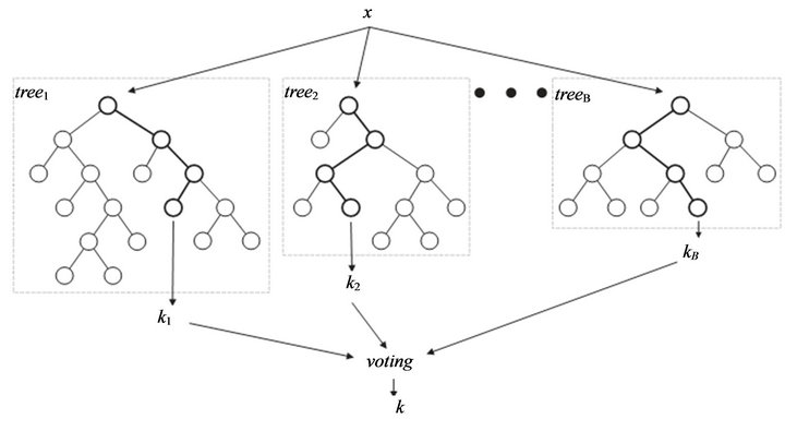
Figure 1. General Architect of random forest.
based components are grown from a certain amount of randomness. Based on this idea, RF is defined as a generic principle of randomized ensembles of decision trees [19]. The basic unit of RF (the so-called base learner) is a binary tree constructed using recursive partitioning (RPART).
The RF tree base learner is typically grown using the methodology of CART [20], a method in which binary splits recursively partition the tree into homogeneous or near homogeneous terminal nodes (the ends of the tree). A good binary split pushes data from a parent tree-node to its two daughter nodes so that the ensuing homogeneity in the daughter nodes is improved from the parent node. RF is often a collection of hundreds to thousands of trees, where each tree is grown using a bootstrap sample of the original data. RF trees differ from CART as they are grown non-deterministically using a two-stage randomization procedure. In addition to the randomization introduced by growing the tree using a bootstrap sample of the original data, a second layer of randomization is introduced at the node level when growing the tree. Rather than splitting a tree node using all variables, RF selects at each node of each tree, a random subset of variables, and only those variables are used as candidates to find the best split for the node. The purpose of this two-step randomization is to de-correlate trees so that the forest ensemble will have low variance, a bagging phenomenon. RF trees are typically grown deeply. In fact, Breiman’s original proposal called for splitting to purity. Although it has been shown that large sample consistency requires terminal nodes with large sample sizes [21], empirically, it has been observed that purity or near purity is often more effective when the feature space is large or the sample size is small. This is because in such settings, deep trees grown without pruning generally yield lower bias. Thus, Breiman's approach is generally favored in genomic analyses. In such cases, deep trees promote low bias, while aggregation reduces variance. The construction of RF is described in the following main steps:
1) Draw ntree bootstrap samples from the original data.
2) Grow a tree for each bootstrap data set. At each node of the tree, randomly select mtry variables for splitting. Grow the tree so that each terminal node has no fewer than nodesize cases.
3) Aggregate information from the ntree trees for new data prediction such as majority voting for classification.
4) Compute an out-of-bag (OOB) error rate by using the data not in the bootstrap sample.
RF [22] can handle thousands of variables of different types with many missing values. Figure 2 presents bootstrapped sample and out of bag sample in random forest algorithm. For a tree grown on a bootstrap data, the OOB data can be used as a test set for that tree. As the number of trees increases, RF provides an OOB data-based unbiased estimate of the test set error. OOB data are also used to estimate importance of variables. These two estimates (test set error estimate and variable importance) are very useful byproducts of RF.
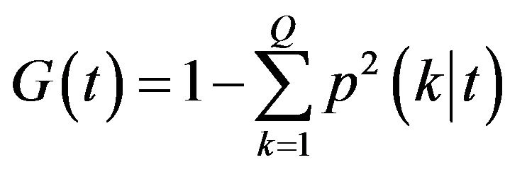
Variable importance: There are four variable importance measures implemented in the RF software code [23,24]. Two measures, based on the GINI index of node impurity and classification accuracy of OOB data, are usually used. Given a node t and estimated class probabilities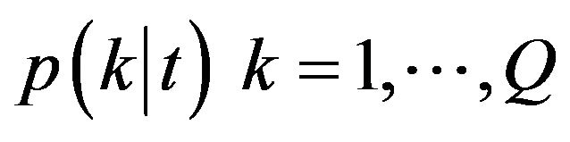 , the Gini index is defined as [25]
 (1)
(1)
where Q is the number of classes.
To calculate the GINI index based measure, at each
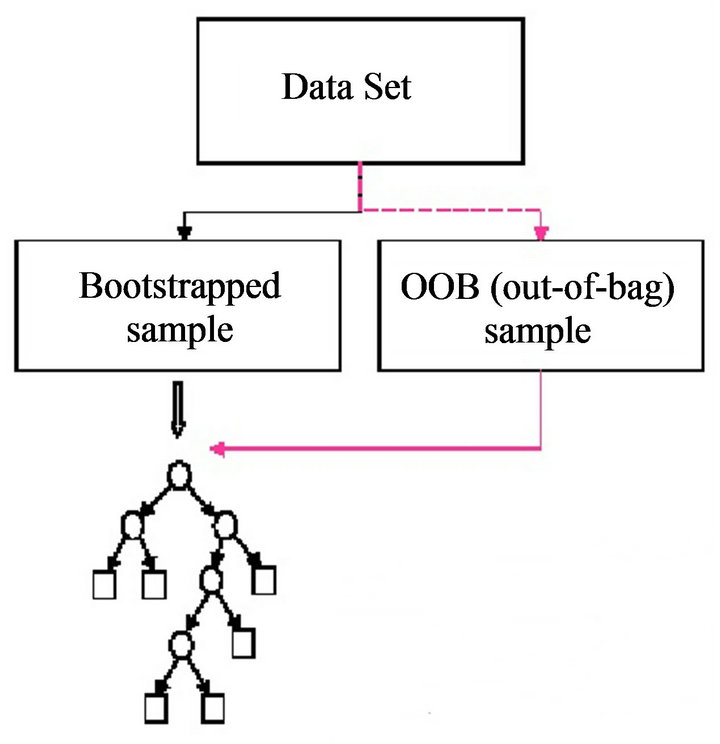
Figure 2. Bootstrapped sample and out of bag sample in random forest.
node the decrease in the GINI index is calculated for variable xj used to make the split. The GINI index-based variable importance measure  is then given by the average decrease in the GINI index in the forest, where the variable xj is used to split a node.
3.2. N-Fold Cross Validation
In n-fold cross validation approach [26-29], we randomly partition into N sets of equal size and run the learning algorithm N times. Each time, one of the N sets is the test set, and the model is trained on the remaining N − 1 sets. The value of K is scored by averaging the error across the N test errors. We can then pick the value of K that has the lowest score, and then learn model parameters for this K. A good choice for N is N = M − 1, where M is the number of data points. This is called Leave-one-out cross-validation.
3.3. Bayesian Probability
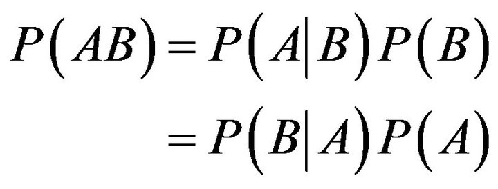
Bayes’ rule [30,31] really involves nothing more than the manipulation of conditional probabilities. As we know, the joint probability of two events, A & B, can be expressed as
 (2)
(2)
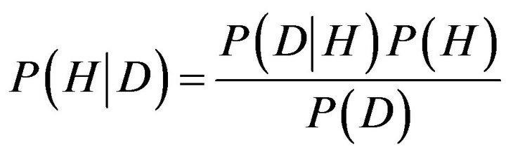
In Bayesian probability theory, one of these “events” is the hypothesis, H, and the other is data, D, and we wish to judge the relative truth of the hypothesis given the data. According to Bayes’ rule, we do this via the relation
 (3)
(3)
The term P(D|H) is called the likelihood function and it assesses the probability of the observed data arising from the hypothesis. Usually this is known by the experimenter, as it expresses one’s knowledge of how one expects the data to look given that the hypothesis is true. The term P(H) is called the prior, as it reflects one’s prior knowledge before the data are considered. The specification of the prior is often the most subjective aspect of Bayesian probability theory, and it is one of the reasons statisticians held Bayesian inference in contempt. But closer examination of traditional statistical methods reveals that they all have their hidden assumptions and tricks built into them. Indeed, one of the advantages of Bayesian probability theory is that one’s assumptions are made up front, and any element of subjectivity in the reasoning process is directly exposed. The term P(D) is obtained by integrating (or summing) P(D|H)P(H) over all H, and usually plays the role of an ignorable normalizing constant. Finally, the term P(D|H)P(H) is known as the posterior, and as its name suggests, reflects the probability of the hypothesis after consideration of the data. Another way of looking at Bayes’ rule is that it represents learning. That is, the transformation from the prior, P(H), to the posterior, P(H|D), formally reflects what we have learned about the validity of the hypothesis from consideration of the data [32,33].
4. PROPOSED METHOD
The proposed method can be understood as a two-phase method. In the phase one, the learning algorithm RF was trained and tested on the training set and validation set in order to select the best features (overall view of the proposed method is presented in Figure 3). The most important procedure in phase one is to estimate feature ranking value for each feature based on Bayesian probability and feature impurity, after that all these features will be rank in ascending order based on feature ranking value. A backward elimination approach was applied to evaluated contribution of each feature to the classifier through oneby-one eliminating feature and comparing classification accuracy before and after eliminating the feature. Output of the phase one is a set of selected features. In the phase two, also on the same dataset only the selected features were used to train the classifier so that classification accuracy was improved.
The proposed method is descripted as four-step classification algorithm as following:
• Step 1: Use n-fold cross validation to training learning algorithm.
◦ Step 2:
◦ Estimate the Bayesian probability;
◦ Estimate the feature ranking value and rank the features.
Step 3:
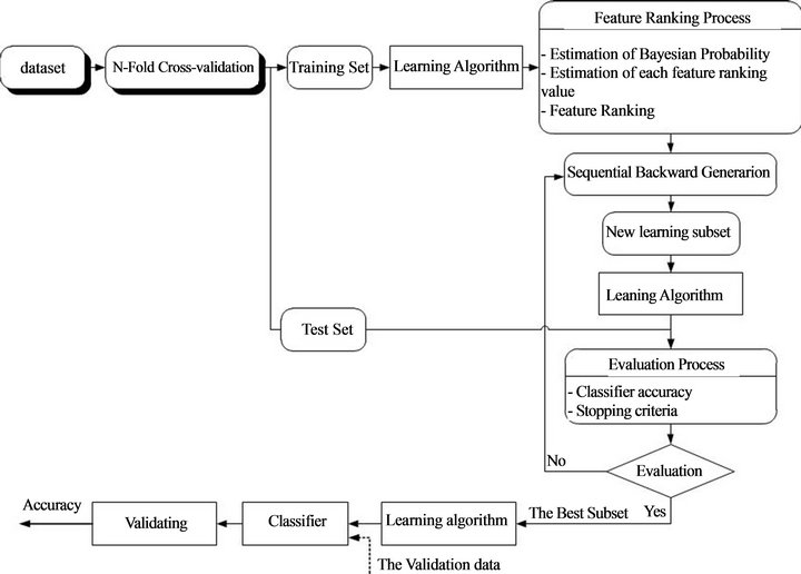
Figure 3. Overall view of the proposed method.
◦ Backward elimination approach to eliminate feature, start from the smallest feature in the feature ranking list;
◦ Evaluate the important of the eliminated feature though variance of classification accuracy with and without eliminating feature. If subtraction of classification accuracy before eliminating the feature and after eliminating the feature is positive then the feature should be kept, otherwise the feature is the redundant feature and it should be deleted.
◦ Step 4:
◦ Check the stopping criteria;
◦ Go to Step 1 if not meet the stopping criteria, otherwise stop the process.
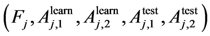
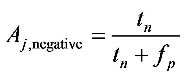
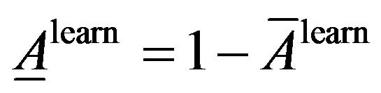
In Step 1 we use n-fold cross validation to train the learning algorithm. In jth cross validation we get the set of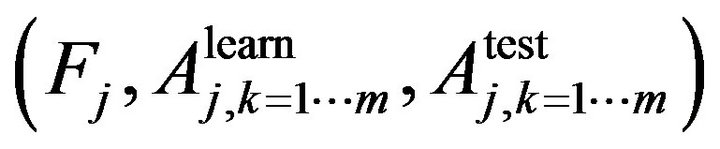 , where
 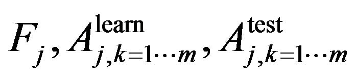 is the trait importance of the learning accuracy of class kth and the test accuracy of class kth respectively. For example, if we need to classify a dataset into two classes, using random forest with n-fold cross validation at jth cross validation we will obtain a set of
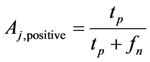
 . The classification accuracy on class kth is calculated as Equation (4) below:
For example, we have a confusion matrix with two classes are positive class and negative class, at jth crossvalidation we have

 (5)
(5)
 (6)
(6)
In Step 2, we will setup a feature ranking formula that is use to rank all features in the dataset. This step is the most important step in our algorithm. It is indispensable to mention that our proposed method uses feature ranking formula as key factor to determine as which feature should be eliminated first. In other words, the feature ranking formula will help us in determining which feature may be a noisy/redundancy feature. If a feature has
|
|

high ranking in the dataset then it will be a useful feature for classifier and otherwise. The weakness of feature ranking formula will lead to the weakness of proposed algorithm because this problem will lead time-consuming and classification accuracy of algorithm. This problem will be discussed in Step 3 in detail.
In reality, a simply method usually will use when we judge whether the feature is useful to the classifier or not. The method can best be understood as follow: we add a feature into the training set; let a learning algorithm learn on the training set; assess classification accuracy on validation set before and after adding the feature. However, in our situation the question is that how can we have a good estimation of classification accuracy? In order to deal with this issue, within the scope of this paper we will use Bayesian probability to estimate classification accuracy.
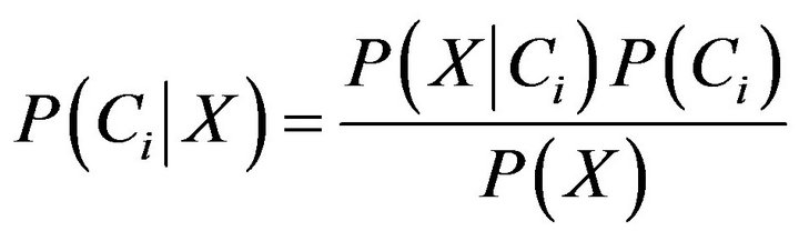
Now assume that there are m classes, . Given an entity X, X is depicted by n features, X = (X1, X2,···,Xn). According to Bayesian probability, the probability that X belongs to the class Ci (I = 1,···,m) is estimated as follow:
 (7)
(7)
P(X) is constant for all classes because we know that the probability of an entity can be classified in to a class are the same, so that only  need to be estimated. According to Bayes’ suggestion in case the prior probabilities of the class are unknown, then it is commonly assumed that prior probabilities of all the classes are equally or in other word we have P(C1) = P(C2) = ··· = P(Cm), and we therefore only need to estimate
  .
.
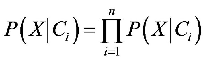
We know that with the given dataset of many attributes, it would be extremely computationally expensive to estimates  . In order to reduce computation in evaluating
 , the naive assumption of conditional independence of class is made. This presumes that the values of the attributes are conditionally independent of one another. Thus,
 (8)
(8)
Or
 (9)
(9)
 (10)
(10)
From (4) and (10) we propose a way to estimate average of classification accuracy and average classification inaccuracy on the learning dataset as following:
Average of classification accuracy:
Average of classification inaccuracy:
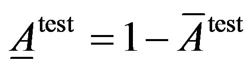
Similarly, average classification accuracy and average classification inaccuracy the on the test dataset:
Average of classification accuracy:

Average of classification inaccuracy:
To evaluate classification accuracy we use fraction of average of classification accuracy and average of classification inaccuracy that are calculated as following.
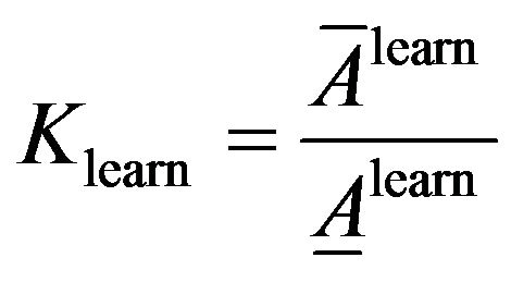 (11)
(11)
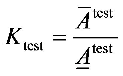 (12)
(12)
We propose a new feature ranking formula for feature ith at jth cross validation as following:
 (13)
(13)
where:
+k = 1,···, n is the number of cross validation folders+Fi,j is GINI index in case of using decision tree algorithms
 and
and  are evaluating parameters of classifier performance on learning set and test setThe feature ranking formula includes two elements: 1) the first element is GINI index, the element decreases for each feature over all trees in the forest when we train data by learning algorithm random forest; 2) the second element is fraction, nominator of the fraction is constant, equals to 1, denominator of the fraction equals
  , presents the variance between classification accuracy on the learning set and the test set. That means the smaller variance, the better features we have. The combination between GINI index and the fraction presents our expectation: higher ranking feature are better feature. After finishing the Step 2, we have an ordered list of ranking features. The list will be used in Step 3 to determine optimal features for the classifier. One should be noted that feature assessing procedure is the correlation among features. We know that a feature may have a low position in feature ranking list but when it is use concurrently with other features they will bring a great contribution to classification accuracy. One feasible way to deal with this issue is to use feature elimination strategy which is the next step (Step 3) of our proposed method.
In Step 3, we use backward elimination approach to eliminate noisy/redundant features. In this step, we will use feature ranking list as a standard criterion to determine which feature should be eliminated first. In this proposed method the feature of lowest position in feature ranking list will be eliminated first. At each step in feature eliminating procedure we will validate the classification accuracy. Purpose of the validation is to determine whether the eliminated feature is actually redundancy/ noisy feature or not. We can perform the validation by comparing the classification accuracy before and after eliminating the feature. If classification accuracy before eliminating feature is greater than that of after eliminating feature then the feature will be kept, otherwise it will be eliminated. This iteration will terminate whenever classification accuracy of new subset is higher than classification accuracy of previous subset. Our algorithm will stop when we cannot find better classification accuracy or no feature to eliminate. In this case the current subset is the best subset we can have. Otherwise, in term of n-fold cross validation the procedure will jump back to Step 1 (Step 4).
5. RESULTS AND DISCUSSION
5.1. Data Description
Two different sets of data have been used taken from the Machine Learning Repository of the University of California, Irvine, USA (ftp://ftp.ics.uci.edu/pub/machine-learning-databases, 2012).
5.1.1. Wisconsin Breast Cancer Diagnosis Dataset
The features of the diagnostic collection describe characteristics of the cell nuclei present in a digitized image of a fine needle aspirate (FNA) of a breast mass [34]. Every cell nucleus is defined by ten traits and for every trait the mean, the standard error and the worst (mean of the three largest values) are computed, resulting in a total of 30 features for each image:
• Radius (mean of distances from center to points on the perimeter): 10.95 - 27.22;
• Texture (standard deviation of gray-scale values): 10.38 - 39.28;
• Perimeter: 71.90 - 182.10;
• Area: 361.60 - 2250;
• Smoothness (local variation in radius lengths): 0.075 - 0.145;
• Compactness (perimeter2/area-1.0): 0.046 - 0.311;
• Concavity (severity of concave portions of the contour): 0.024 - 0.427;
• Concave points (number of concave portions of the contour): 0.020 - 0.201;
• Symmetry: 0.131 - 0.304;
• Fractal dimension (coastline approximation-1): 0.050 - 0.097.
5.1.2. Wisconsin Breast Cancer Prognosis Dataset
The prognostic problem has two outcomes (non-recurrent with 151 samples and recurrent with 47) and has the same 30 attributes measured for breast images in the diagnostic situation, plus three more:
• Time (recurrence time if class is recurrent, diseasefree time if non-recurrent): 1 - 125;
• Tumor size—diameter of the excised tumor in centimeters: 0.400 - 10.00;
• Lymph node status—number of positive axillary lymph nodes observed at time of surgery: 0 - 27.
5.2. Experimental Results
In this section we present experimental results of the proposed method through fifty times of trials. The proposed method for breast cancer diagnosis and prognosis were implemented by using the R program language version 2.1.5.2 with RF package. The both of datasets were divided randomly into training set and validation set in the ratio of 1 to 1.
The parameters of the proposed method in this experiment were determined as follows:
• Number of trees in RF: 25;
• Number of remaining features: 15—the proposed method will be stop if number of remaining features in dataset is greater or equal number of remaining features.
The proposed method was experimented 50 times on both WBCDD and WBCPD. Table 1 shows the results of the proposed method.
Figures 4 and 5 present performances of proposed method on training set and validation set of WBCDD and WBCPD.
Table 2 shows number of original features and number of features were selected. The result indicates that the feature subsets selected by the proposed approach have a better classification performance than that produced by the original RF.
Table 3 presents time-consuming of the proposed method. It should be noted that the proposed method was
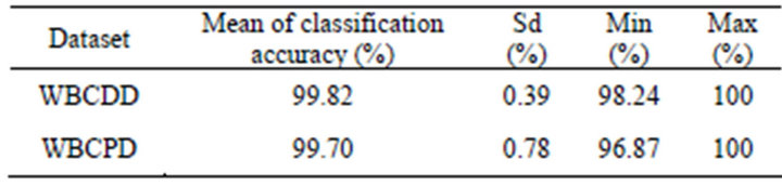
Table 1. Results of 50 trials on WBCDD and WBCPD.
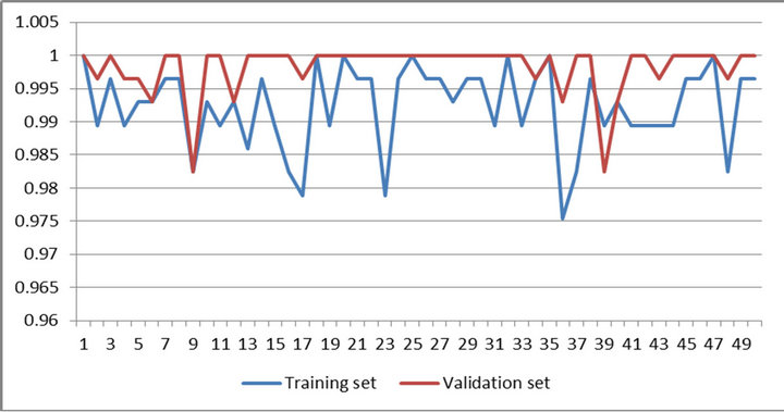
Figure 4. Result of 50 trials of proposed method on training set and validation set of WBCDD.
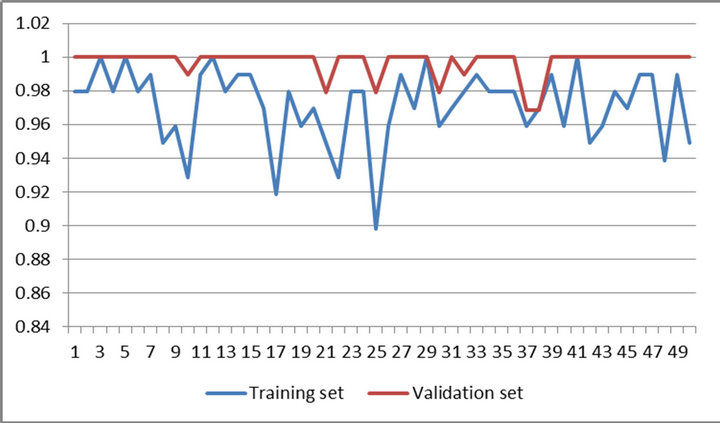
Figure 5. Results of 50 trials of proposed method on training set and validation set of WBCPD.
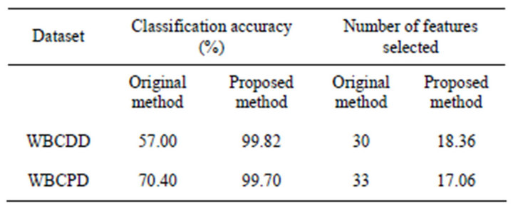
Table 2. A comparison on classification accuracy and number of features selected between original method and proposed method (50 trails).
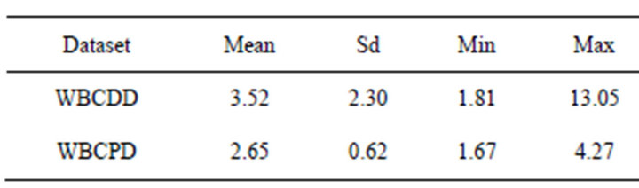
Table 3. Time-consuming (second) of the proposed method (50 trails).
carried out on a laptop computer with the central processing unit Intel Core 2 Duo 2.13 GHz so that timeconsuming is not a challenge of the proposed method.
In this paper ROC is used to evaluate performance of the proposed method. The sensitivity and specificity of the proposed method are presented in Table 4. Figures 6 and 7 show ROC curve those are built based on sensitiv-
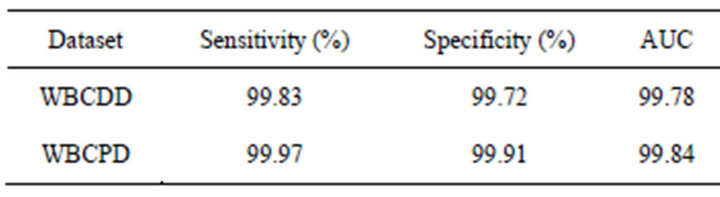
Table 4. The sensitivity and specificity of the proposed method.
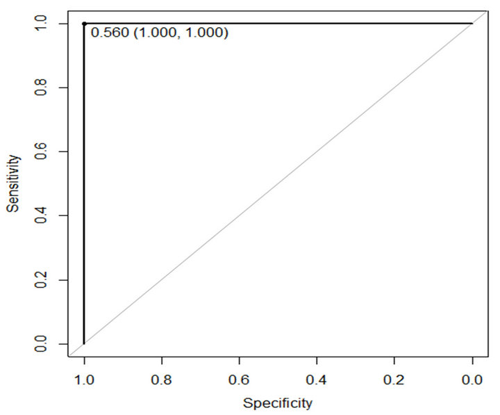
Figure 6. ROC curve of proposed method on WBCDD.
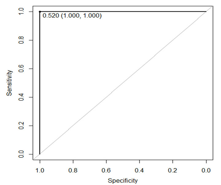
Figure 7. ROC curve of proposed method on WBCPD.
ity and specificity of the propose method on WBCDD and WBCPD, respectively. The results indicate that the proposed method is a reliable diagnostic tool for breast cancer diagnosis and prognostic.
For comparison purposes, Table 5 gives the classification accuracies of our method and previous methods. As we can see from the results, our method obtains the highest classification accuracy so far.
6. CONCLUSIONS
With the non-stop improvements in expert systems and
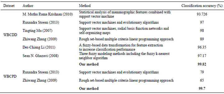
Table 5. Classification accuracies obtained with our proposed system and other classifiers from literature.
machine learning tools, the effects of these innovations are entering to more application domains day-by-day and medical field is one of them. Decision making in medical field can be a trouble sometimes. The expert systems and machine learning tools that are used in medical decision making provide medical data to be examined in shorter time and more detailed. In order to significantly improve predictive accuracy for breast cancer diagnosis and prognosis we developed a classifier model by combining the random forest classifier and feature selection technique. The classification accuracies of the proposed model are 99.82% on WBCDD and 99.7% on WBCPD. From the above results, we conclude that the proposed method obtains very promising results in classifying the possible breast cancer. We believe that the proposed system can be very helpful to the physicians for their as a second opinion for their final decision. By using such an efficient tool, they can make very accurate decisions. Our method is proved to be superior to the state-of-the-art algorithms applied to the Wisconsin Breast Cancer Database, and shows that it can be an interesting alternative.
REFERENCES
- The Women’s Health Resource (2013) What is breast cancer. http://www.imaginis.com/general-information-on-breast-cancer/what-is-breast-cancer-2
- WHO (2012) Breast cancer: Prevention and control. http://www.who.int/cancer/detection/breastcancer/en/index1.html
- UCI Machine Learning Repository (2012) Wisconsin breast cancer dataset. http://archive.ics.uci.edu/ml/datasets.html?format=&task=cla&att=&area=&numAtt=&numIns=&type=&sort=nameUp&view=table
- Chen, H.-L., Yang, B., Liu, J. and Liu, D.-Y. (2011) A support vector machine classifier with rough set-based feature selection for breast cancer diagnosis. Expert Systems with Applications, 38, 9014-9022. doi:10.1016/j.eswa.2011.01.120
- Keles, A., Keles, A. and Yavuz, U. (2011) Expert system based on neuro-fuzzy rules for diagnosis breast cancer. Expert Systems with Applications, 38, 5719-5726. doi:10.1016/j.eswa.2010.10.061
- Marcano-Cedeño, A., Quintanilla-Dominguez, J. and Andina, D. (2011) WBCD breast cancer database classification applying artificial metaplasticity neural network. Expert Systems with Applications, 38, 9573-9579. doi:10.1016/j.eswa.2011.01.167
- Ince, M.C. and Karabatak, M. (2009) An expert system for detection of breast cancer based on association rules and neural network. Expert Systems with Applications, 36, 3465-3469. doi:10.1016/j.eswa.2008.02.064
- Polat, K. and Günes, S. (2007) Breast cancer diagnosis using least square support vector machine. Digital Signal Processing, 11, 694-701. doi:10.1016/j.dsp.2006.10.008
- Ubeyli, E.D. (2007) Implementing automated diagnostic systems for breast cancer detection. Expert Systems with Applications, 33, 1054-1062. doi:10.1016/j.eswa.2006.08.005
- Sahana, S., Polat, K., Kodaz, H. and Günes, S. (2007) A new hybridmethod based on fuzzy-artificial immune system and k-nn algorithmfor breast cancer diagnosis. Computers in Biology and Medicine, 377, 415-423. doi:10.1016/j.compbiomed.2006.05.003
- Abonyi, J. and Szeifert, F. (2003) Supervised fuzzy clustering for the identification of fuzzy classifiers. Pattern Recognition Letters, 24, 2195-2207. doi:10.1016/S0167-8655(03)00047-3
- Quinlan, J.R. (1996) Improved use of continuous attributes in C4.5. Journal of Artificial Intelligence Research, 4, 77-90.
- Krishnan, M.M.R., Banerjee, S., Chakraborty, C., Chakraborty, C. and Ray, A.K. (2010) Statistical analysis of mammographic features and its classification using support vector machine. Expert Systems with Applications, 37, 470-478. doi:10.1016/j.eswa.2009.05.045
- Stoean, R. and Stoean, C. (2013) Modeling medical decision making by support vector machines, explaining by rules of evolutionary algorithms with feature selection. Expert Systems with Applications, 40, 2677-2686. doi:10.1016/j.eswa.2012.11.007
- Mu, T.T. and Nandi, A.K. (2007) Breast cancer detection from FNA using SVM with different parameter tuning systems and SOM-RBF classifier. Journal of the Franklin Institute, 344, 285-311. doi:10.1016/j.jfranklin.2006.09.005
- Zhang, Z.W., Shi, Y. and Gao, G.X. (2009) A rough setbased multiple criteria linear programming approach for the medical diagnosis and prognosis. Expert Systems with Applications, 36, 8932-8937. doi:10.1016/j.eswa.2008.11.007
- Li, D.-C., Liu, C.-W. and Hu, S.C. (2011) A fuzzy-based data transformation for feature extraction to increase classification performance with small medical data sets. Artificial Intelligence in Medicine, 52, 45-52. doi:10.1016/j.artmed.2011.02.001
- Ghazavi, S.N. and Liao, T.W. (2008) Medical data mining by fuzzy modeling with selected features. Artificial Intelligence in Medicine, 43, 195-206.
- Breiman, L. (2001) Random forests. Machine Learning Journal Paper, 45, 5-32.
- Wu, X.D. and Kumar, V. (2009) The top ten algorithm in data mining. Chapman & Hall/CRC, London.
- Biau, G., Devroye, L. and Lugosi, G. (2008) Consistency of random forests and other averaging classifiers. Journal of Machine Learning Research, 9, 2015-2033.
- Verikas, A., Gelzinis, A. and Bacauskiene, M. (2011) Mining data with random forests: A survey and results of new tests. Pattern Recognition, 44, 330-349. doi:10.1016/j.patcog.2010.08.011
- Liaw, A. and Watthew, M. (2002) Classification and regression by random forest. R News, 3, 18-22.
- Breiman, L. (2004). RFtools—For predicting and understanding data. Technical Report. http://oz.berkeley.edu/users/breiman/RandomForests
- Breiman, L., Friedman, J., Stone, C.J. and Olshen, R.A. (1993) Classification and regression tree. Chapman & Hall, London.
- Su, X. (2007) Bagging and random forests. http://pegasus.cc.ucf.edu/~xsu/CLASS/STA5703/notes11.pdf
- Efron, B. (1994) The jackknife, the bootstrap and other resampling plans. 6th Edition, Capital City Press, Baton Rouge, 1994.
- Dupret, G. and Koda, M. (2001) Theory and methodology: Boostrap resampling for unbalanced data in supervised learning. Eropean Journal of Operational Research, 134, 141-156. doi:10.1016/S0377-2217(00)00244-7
- Good, P.I. (2006) Resampling methods: A practical guide to data analysis. 3rd Edition, Birkhauser.
- Hsu, C.-C., Wang, K.-S. and Chang, S.-H. (2011) Bayesian decision theory for support vector machines: Imbalance measurement and feature optimization. Expert Systems with Applications, 38, 4698-4704. doi:10.1016/j.eswa.2010.08.150
- Koch, K.-R. (2007) Introduction to Bayesian statistics. Springer, New York, 2007.
- Brase, C.H. and Brase, C.P. (2012) Understanable statistics. 10th Edition, Cengage Learning, Stamford.
- Hodges, J.J.L. (2005) Basic concepts of probability and statistics. 2nd Edition, Society for Industrial and Applied Mathemtacis, Philadelphia.
- Frank, A. and Asuncion, A. (2010) UCI machine learning repository.
NOTES
*Corresponding author.