Journal of Geographic Information System
Vol.5 No.5(2013), Article ID:38189,6 pages DOI:10.4236/jgis.2013.55045
The Accuracy of GIS Tools for Transforming Assumed Total Station Surveys to Real World Coordinates
1Landscape Architecture Department, KAU, Jeddah, Saudi Arabia
2Civil Engineering Department, Assiut University, Assiut, Egypt
Email: khalilragab@yahoo.com
Copyright © 2013 Ragab Khalil. This is an open access article distributed under the Creative Commons Attribution License, which permits unrestricted use, distribution, and reproduction in any medium, provided the original work is properly cited.
Received August 15, 2013; revised September 7, 2013; accepted September 9, 2013
Keywords: Control Network; Topographic Surveying; Coordinate Transformation; Spatial Adjustment; Georeferencing; CHaMP; Accuracy; Total Station
ABSTRACT
Most surveying works for mapping or GIS applications are performed with total station. Due to the remote nature of many of the sites surveyed, the surveys are often done in unprojected, local, assumed coordinate systems. However, without the survey data projected in real world coordinates, the range of possible analyses is limited and the value of existing imagery, elevation models, and hydrologic layers cannot be exploited. This requires a transformation from the local assumed to the real world coordinate systems. There are various built-in and add-in tools to perform transformations through GIS programs. This paper studies the effect of using Georeferencing tool, Spatial Adjustment tool (Affine and similarity) and CHaMP tool on the precision and relative accuracy of total station survey. This transformation requires real-world coordinates of at least two control points, which can be collected from different sources. This paper also studies the effect of using geodetic GPS, hand-held GPS, Google Earth (GE) and Bing Basemaps as sources for control points on the precision and relative accuracy of total station survey. These effects have been tested by using 111 points covered area of 60,000 m2 and the results have shown that the CHaMP tool is the best for preserving the relative accuracy of the transformed points. The Georeferencing and spatial adjustment (similarity) tools give the same results and their accuracy are between 1/1000 and 1/300 depending on the source of control points. The results have also shown that the cornerstone to preserve the precision and relative accuracy of the transformed coordinates is the relative position of the control points despite their source.
1. Introduction
Total station surveys are a widely used method to survey topography [1], with applications ranging from traditional land surveying [2], land form evolution monitoring [3], to land use monitoring [4]. In the geosciences and biological sciences, total stations are now becoming standard tools in monitoring geomorphic change detection of rivers [5-7], streams [8], beaches [9,10] and mass wasting of hill slopes [11,12]. Since many total station surveys are now undertaken in remote and/or undeveloped localities, there is often not an established local control network tied to a projected real world coordinate system [13]. Thus, many of these surveys are done from an unprojected local assumed coordinate system. However, as GIS has become more of an everyday tool for visualizetion, modeling and analysis of topographic data [3], there is an increasing demand for such surveys to be in real world coordinate system. Transforming total station surveys from unprojected local assumed coordinate system to real world coordinates makes the power of overlaying those data with other datasets (e.g., aerial imagery, vector datasets of roads, political boundaries, etc.) and certain analyses possible. There are various built-in and add-in tools to perform transformations through GIS programs. This paper studies the effect of using Georeferencing tool, Spatial Adjustment tool (Affine and similarity) and CHaMP tool on the precision and relative accuracy of total station survey. This transformation requires real-world coordinates of at least two control points, which can be collected from different sources. This paper also studies the effect of using geodetic GPS, hand-held GPS, Google Earth (GE) and Bing Basemaps as sources for control points on the precision and relative accuracy of total station survey.
2. Transformation Methods
There are numerous transformation methods for transforming between coordinate systems ranging from simple to sophisticated. The choice of appropriate method depends on the specifics of the application and is generally one that should be made by someone with proper training in surveying and geomatics as well as a solid understanding of the source data and how it was collected [13]. In this paper, the transformation tools built in ArcGIS (e.g. spatial adjustment tool and georeferencing tool), and add-in tools such as CHaMP tool were used to transform unprojected total station precise observations into projected real world coordinates. All of these tools use affine transformation. An affine transformation is any transformation that preserves collinearity (i.e., all points lying on a line initially still lie on a line after transformation) and ratios of distances. In general, an affine transformation is a composition of rotations, translations, dilations (scales), and shears (skews) [14]. The transformation functions are based on the comparison of the coordinates of source and destination points, also called control points.
2.1. Spatial Adjustment Tool
Spatial adjustment supports a variety of adjustment methods (Transformation, Rubbersheet and edge snap) and will adjust all editable data sources. The affine and similarity transformations were used in this study as they are the appropriate methods to transform total station surveys to real world coordinates.
2.1.1. Affine Transformation
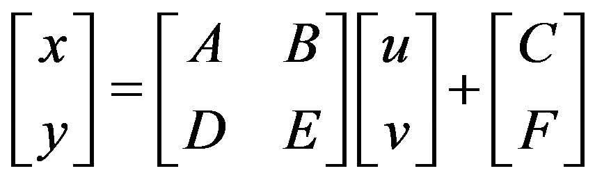
The Affine transformation can be represented by the following equations (in matrix formation) [15].
 (1)
(1)
 (2)
(2)
 (3)
(3)
Where:
u, v are coordinates of the input data and x, y are the transformed coordinates.
A, B, C, D, E, and F are six unknowns; determined by comparing the location of source and destination control points.
Affine transformation can differentially scale the data, skew it, rotate it, and translate it. As there are six unknowns in the transformation equations, this method requires a minimum of three control points.
2.1.2. Similarity Transformation
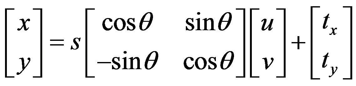
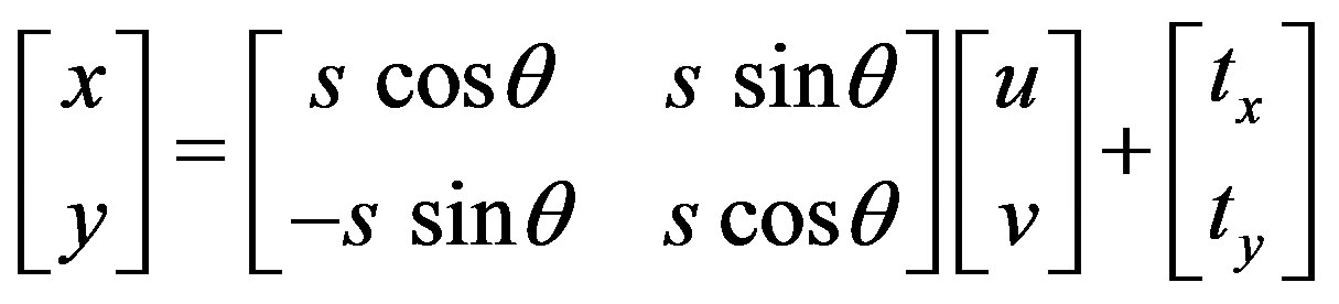
The similarity transformation scales, rotates, and translates the data. It will not independently scale the axes, nor will it introduce any skew. It maintains the aspect ratio of the features transformed, which is important if you want to maintain the relative shape of features. The similarity transformation function (in matrix formation) [15] is:
 (4)
(4)
 (5)
(5)
 (6)
(6)
In similarity method, the scale is the same in both x and y directions, and a minimum of two control points are required.
2.2. Georeferencing Tool
Georeferencing tool is used to adjust raster data using different polynomial equations and to adjust a CAD dataset using the similarity transformation method. The transformation functions are similar to Equations (4)-(6).
2.3. CHaMP Tool
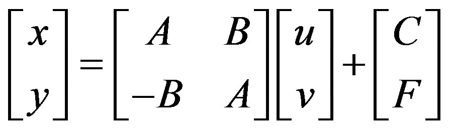
ChaMP tool was introduced by [13]. It uses a simple affine transformation that just rotates and translates the data. This type of transformation is accurate because the scale is preserved [16]. The equations can be as the followings:
 (7)
(7)
 (8)
(8)
This tool requires two control points but three is essentials as stated by the designers.
3. Control Points
To transform the unprojected total station survey data, coordinates in a projected real world coordinate system for two to three control points which were established and used in the total station survey are required. The rotation is performed about one of these points, where the rotation is computed based on the difference in azimuth between point pairs whose coordinates are known in both systems. The origin shift is computed from the rotation point’s coordinates in both systems [16].
There are multiple methods to acquire the real world coordinates of these control points. The most accurate is to use a known pre-existing control network surveyed in real world coordinate system [1,17]. At the same level of accuracy, a geodetic GPS can be used to obtain accurate coordinates for the control points. The problems of these two methods as stated by [13] are that many practitioners often do not have access to geodetic GPS receivers or may not have access to the necessary post-processing software and may work in areas far away of existing control network. Google Earth is a low-cost and readily accessible tool with relatively good spatial accuracy [18, 19]. It offers high resolution imagery from which, it may be possible to derive sufficient quality photo control points if ground features visible in the photo (e.g., fence corner, rockedge, etc.) can be accurately located in the field. The latest versions of ArcGIS offer a high resolution Bing Basemaps which can also be used to drivephoto control points ifground features visible in the photo can beaccurately located in the field. The most common is to use a simple, inexpensive, consumer-grade GPS (e.g., Garmin hand held, Smart-Phone, GPS card in field data collector. The accuracy of such devices is sufficient for purposes of GIS overlay at scales of 1:1000 or coarser [13].
4. Field Data
Topcon total station GPT-7501 was used to collect the coordinates of more than 100 point in a parking and open space area in King Abdulaziz University campus. The total station was first set up on a point with assumed coordinates. Then the total station was oriented with “backsight azimuth” setup which uses bearing to the backsight point, using assumed bearing for the line connected the two points. Once the survey is begun on this assumed coordinate system, all additional station setups and all data, including three control points (which acquired during the survey course), collected in a single unprojected local assumed coordinate system. The collected data was exported to *.txt and once again to *.dxf. The *.txt file was used to generate shapefile while the *.dxf file represents the CAD file. Both files are needed to apply the transformation on.
The projected coordinates of the three control points were collected using four methods 1) RTK GPS with two Topcon GR3 geodetic receivers; one receiver was setup on existing control point at the university main gate while the other receiver was used to acquire the needed points; 2) Garmin handheld GPS; 3) Google Earth at Eye altitude equal to 50 m; and 4) Bing Imagery that is available in ArcGIS as an online basemap layer at scale 1:100.
5. Results and Discussion
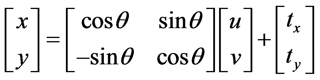
To check the accuracy of coordinate transformation tools available in ArcGIS, the relative position of surveyed points were calculated before and after transformation using the different tools and compared to the original positions. The most upper left point was chosen as an origin and the distances from it to all other points were computed using the raw data and data after transforming the coordinates. The difference between distances to the corresponding points were calculated and represented in Figure 1 for control points acquired using geodetic GPS. Figures 2-4 represent the errors in relative positions for control points collected using Bing basemap imagery, Google Earth and Hand-held GPS respectively.
From the figures it’s clear that there are no errors in
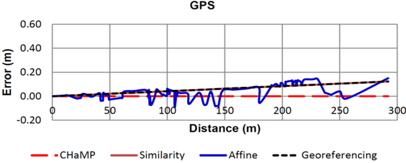
Figure 1. Relative error in point positions using GPS control points.
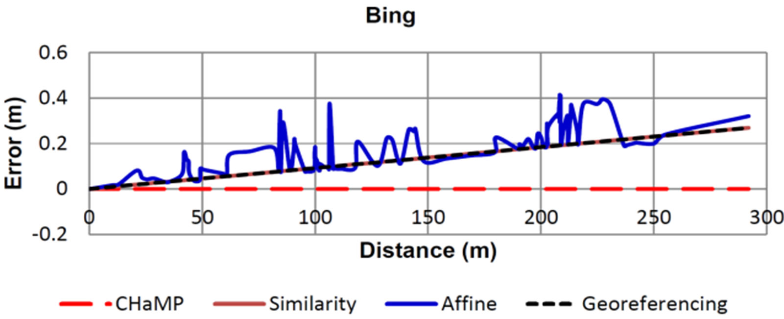
Figure 2. Relative error in point positions using Bing basemap control points.
Figure 3. Relative error in point positions using Google Earth control points.

Figure 4. Relative error in point positions using Gamin GPS control points.
coordinates transformed using CHaMP tool regardless the source of the control points. The errors in coordinates resulting using Georeferencing tool and Spatial Adjustment tool (similarity) are the same, and the error increases as the distance from the origin increases. The error at the farthest point was 0.12 m, 0.27 m, 0.45 m and 0.99 m for GPS, Bing basemap, Google Earth and Garmin control points respectively. The error ratios were 1:2400, 1:1100, 1:650 and 1:300 respectively. Errors in coordinates due to using Spatial Adjustment tool (Affine) are undulated and its trend is almost the same as Georeferencing and similarity transformation.
CHaMP tool uses simple mathematical operation of a translation and rotation, so it preserves the relative positional accuracy and precision of the total station survey. The data may be shifted out of its absolute location depending on the absolute accuracy of the control points. A single control point will ultimately be used as the basis for the horizontal translation and datum adjustment, and a bearing based on a second control point will be used to define the rotation [13].
To explain the results of the other tools, let’s first have a look on the absolute coordinates of the control points acquired from the different sources which shown in Table 1 and the deviations in these coordinates related to the GPS points as it is the most accurate which shown in Table 2.
From Table 2, one can notice that GE points are much closer to GPS points than Bing points, while Figures 2 and 3 show that errors in the transformed coordinates using GE points are bigger than those resulted when using Bing points. This means that the absolute location of control points does not affect the transformation accuracy.
The distances between control points are shown in Table 3, and the deviations from the original (total station) distances are shown in Table 4.
From Table 4, the error in distance (1-2) between control points (1) and (2) increases from GPS to Bing to GE to Garmin. Spatial Adjustment (Similarity) and Georeferencing tools use two control points to transform the coordinates. These tools preserve the relative geometry of the control points and scale (stretch) the source data to fit the geometry of the controls. This explains increasing the error in the transformed coordinates according to the increase of that distance error as shown in Figures 1-4. These two transformation tools scale the coordinates with the same amount in both X and Y axes, so the error in the transformed coordinates of any point is proportional to the distance to that point from the base control point.
Spatial Adjustment (Affine) tool uses and preserve the relative geometry of three control points, so this tool stretch and skew the source data. The trend of the error in the relative position of the transformed data is due to the error in distance (1-2), while the undulations of error chart is due to the error in distance (1-3) as shown in Figures 1-4. The error in distance (1-2) for Bing is smaller than that of GE, so the trend of error in transformed data using Bing control points is smaller than that for GE control points as shown in Figures 2 and 3. The distance (1-3) for Bing is greater than that of GE, accordingly the error in relative positions due to using Bing control points is higher than the error due to using GE control points in transformation. The error in relative position of transformed data depending on the point location related to the line connecting the first two control points as shown in Figure 5, which show that the maximum error is in the points far away from the mentioned line.
6. Conclusions
From the results and discussion, the followings could be concluded:
1) CHaMP transformation tool uses a simple rotation and translation transformation to preserve the precision and relative accuracy of the total station survey.
2) Georeferencing and Spatial Adjustment similarity transformation tools preserve the location of the two control points used in the transformation, so they stretch the data and introduce errors in point location depending on the relative position of the control points.
3) Spatial Adjustment Affine transformation tool preserves the location of the three control points used in the transformation, so it stretches and warps the data which introduce errors in point location depending on the relative position of the control points and on the point location related to the line connect the first two control points.
4) The cornerstone of the accuracy of build in transformation tools is the relative positions of the control points.
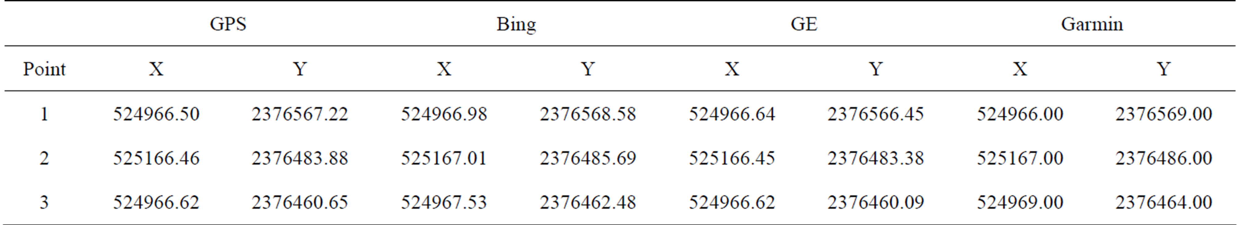
Table 1. The absolute coordinates of the control points.
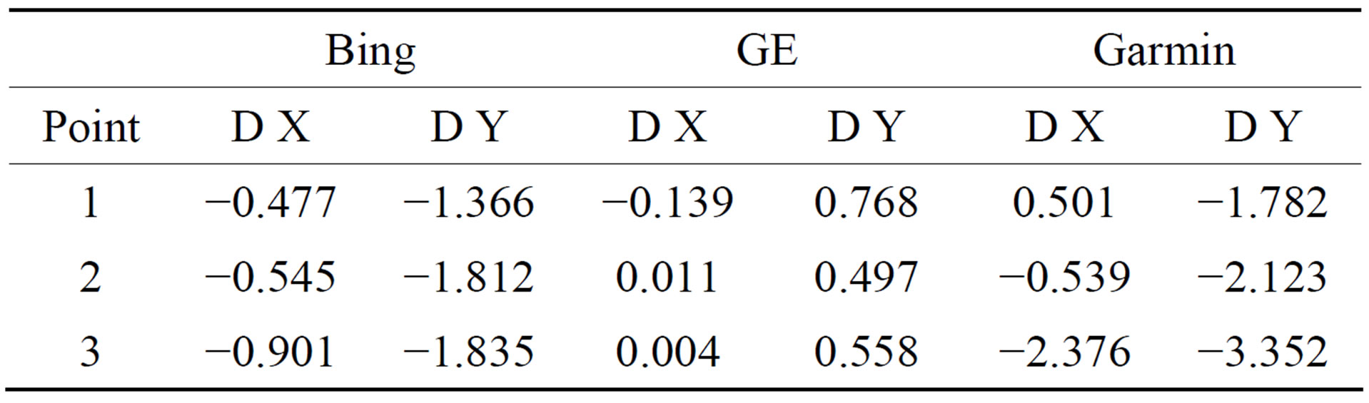
Table 2. The deviations in coordinates from GPS points.
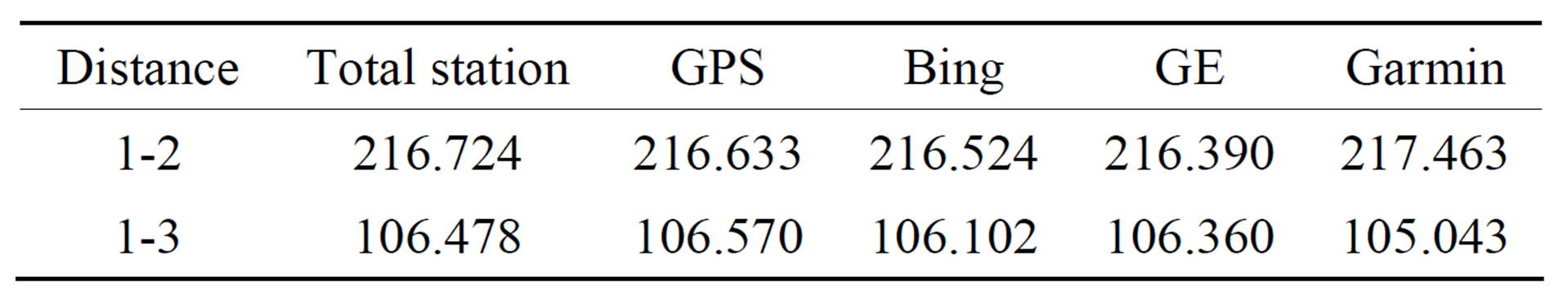
Table 3. Distances between control points.
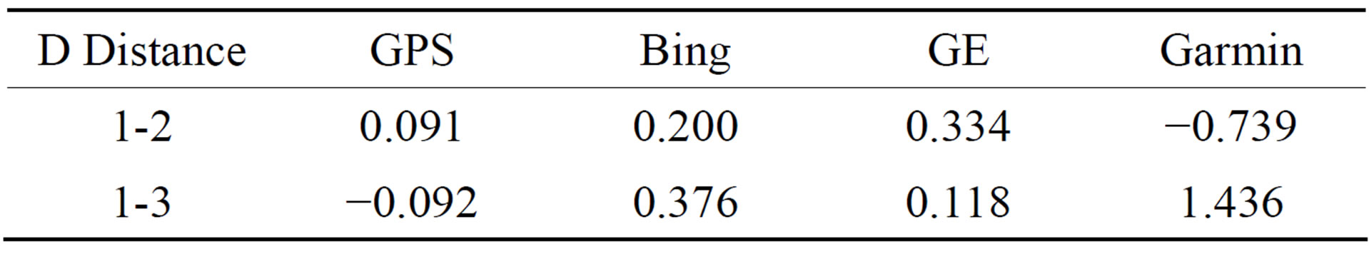
Table 4. The deviations from the original distance.
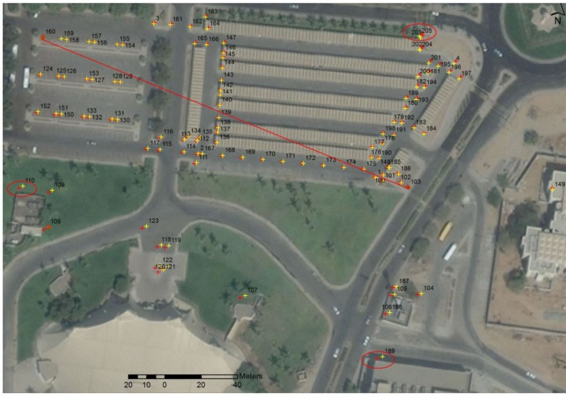
Figure 5. Location of maximum errors due to affine transformation tool.
7. Acknowledgements
Thanks are due to Mr. Talal Al-Thebety for assistance in performing the field measurements.
REFERENCES
- USACE, “Control and Topographic Surveying,” Engineering Manual, EM1110-1-1005, US Army Corps of Engineers, Vicksburg, 2007, 498 p.
- U. Kizil and L. Tisor, “Evaluation of RTK-GPS and Total Station for Applications in Land Surveying,” Journal of Earth System Science, Vol. 120, No. 2, 2011, pp. 215- 221. http://dx.doi.org/10.1007/s12040-011-0044-y
- S. N. Lane and J. H. Chandler, “Editorial: The Generation of High Quality Topographic Data for Hydrology and Geomorphology: New Data Sources, New Applications and New Problems,” Earth Surface Processes and Landforms, Vol. 28, No. 3, 2003, pp. 229-230. http://dx.doi.org/10.1002/esp.479
- L.-S. Lin, “Application of GPS RTK and Total Station System on Dynamic Monitoring Land Use,” The XXth ISPRS Congress, Istanbul, July 2004, pp. 12-23.
- S. N .Lane, J. H. Chandler and K. S. Richards, “Developments in Monitoring and Modeling Small-Scale River Bed Topography”, Earth Surface Processes and Landforms, Vol. 19, No. 4, 1994, pp. 349-368. http://dx.doi.org/10.1002/esp.3290190406
- I. C. Fuller, A. R. G. Large and D. J. Milan, “Quantifying Channel Development and Sediment Transfer Following Chute Cutoff in a Wandering Gravel-Bed River,” Geomorphology, Vol. 54, No. 3-4, 2003, pp. 307-323. http://dx.doi.org/10.1016/S0169-555X(02)00374-4
- J. E. Merz, G. B. Pasternack and J. M. Wheaton, “Sediment Budget for Salmonid Spawning Habitat Rehabilitation in a Regulated River,” Geomorphology, Vol. 76, No. 1-2, 2006, pp. 207-228. http://dx.doi.org/10.1016/j.geomorph.2005.11.004
- D. M. Walters, D. S. Leigh, M. C. Freeman, B. J. Freeman and C. M. Pringle, “Geomorphology and Fish Assemblages in a Piedmont River Basin, USA,” Fresh-Water Biology, Vol. 48, No. 11, 2003, pp. 1950-1970. http://dx.doi.org/10.1046/j.1365-2427.2003.01137.x
- I. Delgado and G. Lloyd, “A Simple Low Cost Method for One Person Beach Profiling,” Journal of Coastal Research, Vol. 20, No. 4, 2004, pp. 1246-1253. http://dx.doi.org/10.2112/03-0067R.1
- P. Baptista, T. R. Cunha, A. Matias, C. Gama, C. Bernardes and O. Ferreira, “New Land-Based Method for Surveying Sandy Shores and Extracting DEMs: The INSHORE System,” Environmental Monitoring and Assessment, Vol. 182, No. 1-4, 2011, pp. 243-257. http://dx.doi.org/10.1007/s10661-011-1873-5
- J. J. De Sanjose-Blasco, A. D. J. Atkinson-Gordo, F. Salvador-Franch and A. Gomez-Ortiz, “Application of Geomatic Techniques to Monitoring of the Dynamics and to Mapping of the Veleta Rock Glacier (Sierra Nevada, Spain) ,” Zeitschrift Fur Geomorphologie, Vol. 51, 2007, pp. 79-89. http://dx.doi.org/10.1127/0372-8854/2007/0051S2-0079
- B. H. Mackey, J. J. Roering and J. A. McKean, “LongTerm Kinematics and Sediment Flux of an Active Earthflow, Eel River, California,” Geology, Vol. 9, No. 37, 2009, pp. 803-806.
- J. M. Wheaton, C. Garrard, K. Whitehead and C. Volk, “A simple, Interactive GIS Tool for Transforming Assumed Total Station Surveys to Real World Coordinates—The CHaMP Transformation Tool,” Computers & Geosciences, Vol. 42, 2012, pp. 28-36. http://dx.doi.org/10.1016/j.cageo.2012.02.003
- E. W. Weisstein, “Affine Transformation,” From MathWorld—A Wolfram Web Resource, 1 May 2013. http://mathworld.wolfram.com/AffineTransformation.html
- R. E. Deakin, “Coordinate Transformations in Surveying and Mapping,” Geospatial Science, 2004. http://user.gs.rmit.edu.au/rod/files/publications/COTRAN_1.pdf
- W. Sprinsky, “Transformation of Survey Coordinates: Another Look at an Old Problem,” Journal of Surveying Engineering, Vol. 128, No. 4, 2002, pp. 200-209. http://dx.doi.org/10.1061/(ASCE)0733-9453(2002)128:4(200)
- USACE, “Topographic Surveying,” USA Rmy Corps of Engineers, Washington DC, 111 p. http://www.novaregion.org/DocumentCenter/Home/View/756
- D. Kaimaris, O. Georgoulab, P. Patiasb and E. Stylianidis, “Comparative analYsis on the Archaeological Content of Imagery from Google Earth,” Journal of Cultural Heritage, Vol. 12, No. 3, 2011, pp. 263-269. http://dx.doi.org/10.1016/j.culher.2010.12.007
- N. Q. Chien and S. K. Tan, “Google Earth as a Tool in 2-Dhydrodynamic Modeling,” Computers & Geosciences, Vol. 37, No. 1, 2011, pp. 38-46. http://dx.doi.org/10.1016/j.cageo.2010.03.006