Intelligent Control and Automation
Vol.4 No.2(2013), Article ID:31739,14 pages DOI:10.4236/ica.2013.42021
Modeling and Adaptive Control of an Omni-Mecanum-Wheeled Robot
Department of Mechanical Engineering, National Chung Hsing University, Taichung, Chinese Taipei
Email: lclin@mail.nchu.edu.tw
Copyright © 2013 Lih-Chang Lin, Hao-Yin Shih. This is an open access article distributed under the Creative Commons Attribution License, which permits unrestricted use, distribution, and reproduction in any medium, provided the original work is properly cited.
Received December 14, 2012; revised February 6, 2013; accepted February 13, 2013
Keywords: Mecanum-Wheeled Mobile Robot; Dynamics Model; Backstepping Adaptive Control; Lyapunov Stability
ABSTRACT
The complete dynamics model of a four-Mecanum-wheeled robot considering mass eccentricity and friction uncertainty is derived using the Lagrange’s equation. Then based on the dynamics model, a nonlinear stable adaptive control law is derived using the backstepping method via Lyapunov stability theory. In order to compensate for the model uncertainty, a nonlinear damping term is included in the control law, and the parameter update law with σ-modification is considered for the uncertainty estimation. Computer simulations are conducted to illustrate the suggested control approach.
1. Introduction
In 1973, BengtIlon invented the Mecanum wheel (also called Ilon wheel) when he was an engineer with the Swedish company Mecanum A.B. [1,2]. The Mecanum wheel is designed with passive rollers mounted around the wheel circumference at an angle of 45 degrees to the wheel plane, thus it allows for in place rotation with small ground friction and low driving torque. Usually the mobile robots using Mecanum wheels, such as an intelligent wheelchair, a forklift, or the URANUS omni-directional robot, are designed with four wheels to provide agile mobility in any direction without changing its orientation. This omni-directional capability provides greater flexibility in congested environments. Ould-Khessal [3] applied it in a robot soccer team design.
Although the benefit of omni-directionality of a standard Mecanum wheel, it has an unfortunate side effect of reducing the motor effective driving force through the rollers by projecting a portion of the motor force into a force perpendicular or at an angle to that produced by the motor. Thus, it may be inefficient when the platform travels in a straight line, especially when travels diagonally. Diegel et al. [4] proposed an improved Mecanum wheel design with a “twist” mechanism for adjusting and locking the angle of the passive rollers to best suit the direction the platform is traveling in. Since a planar mobile robot consisting of four Mecanum wheels has only three degrees of freedom (DOF): two translational motions along Xand Y-axes, and one rotation about Z-axis, it has one redundant degree of freedom. Asama et al. [5] proposed a transmission mechanism such that four wheels can be driven by only three actuators, each of which drives wheels to move the robot for a certain DOF, respectively.
The most popular approach to the control of an omnidirectional robot considers the kinematic control relying only on the kinematics model of the platform [e.g. 6,7]. The kinematic control neglects the dynamics effect and thus lowers the effective moving speed that could be obtained. Based on the Newton’s second law, Tlale and de Villiers [8] developed and verified a dynamic model for the omni-directional robot with four Mecanum wheels using the resolved force method. In their developed mobile platform, each wheel was fitted with encoder for measuring the wheel rotation/velocity, and 3D gyrometer and accelerator are also installed in the platform for measuring its orientation and translation motion. Viboonchaicheep et al. [9] presented a position rectification method including symptomatic and preventive rectifications during the position and orientation control. Their control system is based on kinematics and joint-space linear dynamics model. Recently, Han et al. [10], Park et al. [11], and Tsai and Wu [12] proposed fuzzy control systems for Mecanum wheeled robots based on kinematic model or joint-space dynamic model.
In this work, we will propose a more complete kinematics and dynamics modeling of an omni-directional mobile robot with four Mecanum wheels considering both the friction and load eccentricity effects. After establishing the kinematics model, the 3-DOF dynamics model in the Cartesian space is derived using the Lagrange’s equation, which can be used for arbitrary translational and rotational dynamic control. Then an adaptive control is constructed using the backstepping method via Lyapunov stability theory. The derived adaptive controller with uncertainty compensator has excellent three-axis arbitrary trajectory tracking performance, even the platform is encountered a not small eccentricity uncertainty. Finally, simulation results are presented to illustrate the suggested control system performance. The suggested nonlinear controller is more complex than traditional PID control, however it could have more satisfactory and faster arbitrary-trajectory tracking capability.
2. Kinematics and Dynamics Modeling of a Mecanum-Wheeled Mobile Robot
As shown in Figure 1, a Swedish wheel consists of a fixed standard wheel with passive rollers attached to the wheel circumference. The Mecanum wheel is a type of Swedish wheels with , where
  is the angle between the passive-roller rotation axis and the wheel plane. Complete kinematics and dynamics modeling of an omni-directional robot with four Mecanum wheels will be considered in this section.
2.1. Kinematics of a Four-Wheeled Mecanum Robot
Consider a Mecanum wheel mounted on a mobile robot with local coordinate frame {R}: , as shown in Figure 1, where point A is its center and the other geometric parameters are defined as follows.
  is the angle of the vector
 , from the robot frame origin G to the wheel center A, with respect to the
  axis, and
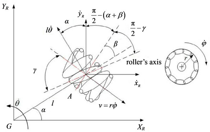
Figure 1. Parameters of a mecanum wheel.
is the angle between the vector  and the main wheel axis. The distance from the geometric center G to the wheel center A is l, and the main wheel’s radius is r. And
  and
and  are respectively the rotation speeds of the main wheel and the passive roller contacted with the flat floor.
Assume that the contact point between the Mecanum wheel and the floor is an instantaneous rotation center, that is, the contact is in a pure rolling condition without slipping, then the corresponding velocity of the wheel center A is  along the tangential direction as shown in Figure 1. So the wheel center A’s velocity component along the contact roller’s axis is
 .
.
Let the robot’s instantaneous translation velocity in terms of local frame {R} be , and the rotation velocity about
  axis be
 . Then the wheel center A’s velocity can also be computed by summing the translational velocity vectors
  and the relative velocity
  due to the rotation velocity shown in Figure 1. Thus, the wheel center A’s velocity component along the contact roller’s axis can be expressed as follows (computed via the platform’s velocity):
 (1)
(1)
If no slipping occurs along the contact roller’s axis, the same velocity can also be computed from the wheel’s rotation speed  Hence, we have the following constraint equation for a Swedish wheel:
 (2)
(2)
Since the rotation matrix representing the orientation of the inertia frame {I} with respect to the robot frame {R} can be expressed as
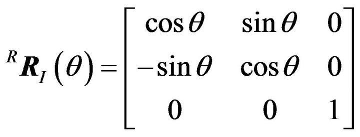 where
where  is the angle between axes
 , and the robot’s velocity vector in terms of the robot frame {R},
 can be computed as:
 where
where  is the robot velocity vector in terms of the inertia frame {I}, Equation (2) can be transformed to as follows [6]:
 (3)
(3)
In the direction orthogonal to the contact roller’s axis, the motion is not constrained because of the free rotation of the passive contact roller, thus we have the following velocity relation:

Thus, the above rolling condition can be transformed as:
 (4)
(4)
Consider the omni-directional robot with four Mecanum wheels shown in Figure 2. The angles  of the mounted four Mecanum wheels,
  are shown in Table 1. From Equation (3), we have the following four constraint equations for the centers of the four Mecanum wheels:
 (5)
(5)

Figure 2. A four-Mecanum-wheeled robot.
Assuming that each Mecanum wheel has equal radius and mounting distances,  and by substituting the parameters in Table 1 into Equation (5), we can obtain the inverse kinematics equation as follows:
 (6)
(6)
where 
Define the Jacobian matrix as:
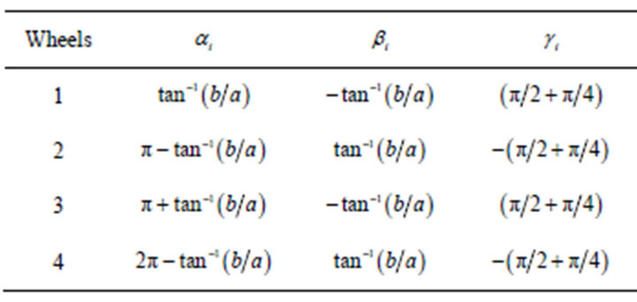
Table 1. Parameters of the Mecanum wheels.
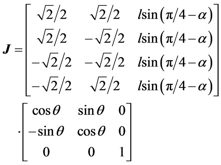 (7)
(7)
The forward kinematics equation of the four-wheeled Mecanum mobile robot can be obtained as follows:
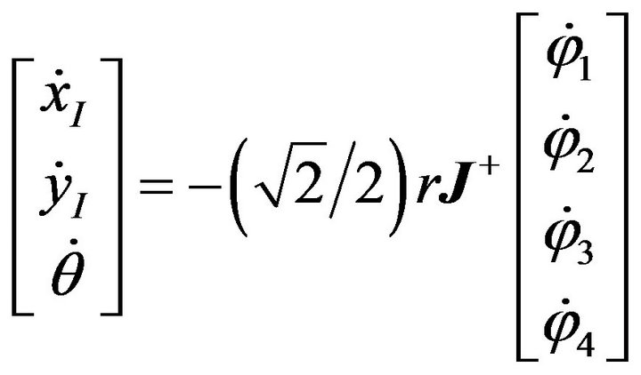 (8)
(8)
where  is the pseudoinverse of J.
2.2. Dynamics of the Mecanum Robot
Consider the four-wheeled Mecanum mobile robot shown in Figure 3, where G is the geometric center with position vector  in terms of the inertia frame {I}, and
  is the mass center of the moving platform with relative position vector
in terms of robot frame {R}. The velocity  of point G, in terms of robot frame {R} can be expressed as
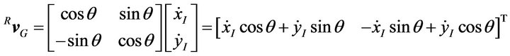 (9)
(9)
where  are the velocity components of G along the
  axes, respectively, and
  is the orientation angle of the platform relative to the reference frame {I}. Hence the velocity
  of the mass center
  in terms of robot frame {R} can be obtained as follows:
 (10)
(10)
The total kinetic energy T of the mobile robot including those of the platform and four Mecanum wheels can be computed as below:
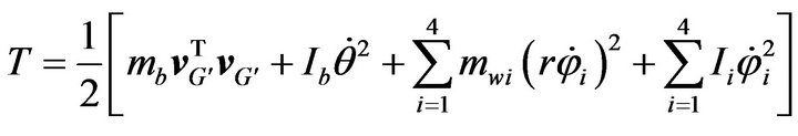 (11)
(11)
where  is the mass of the platform, and
  is the mass of the ith wheel,
 ;
;  is the moment of inertia of the platform about
  axis ( parallel to
 ) through point
 , and
, and  is the moment of inertia of the ith wheel about its main axis;
  is the rotational speed of the platform, and
  is the rotational speed of the ith wheel about its main axis; and
  is the radius of each Mecanum wheel. Since the mobile robot is assumed moving in a plane, the total potential energy
 . Assume that the four Mecanum wheels are identical and thus let
  and
and 
 After substituting Equation (2) and some computations, the Lagrangian
  can be obtained as below:
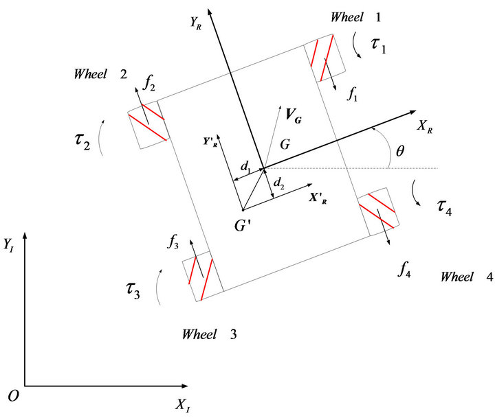
Figure 3. Schematic of the Mecanum robot.
 (12)
(12)
The dynamics model can then be derived using the Lagrange’s equations:
 (13)
(13)
where  is the ith generalized coordinate, and
  is the ith generalized force/torque. The generalized coordinate vector of the mobile robot can be defined as:
 . Refer to Figure 3, where
  is the contact friction force of the ith Mecanum wheel with the floor, the generalized force/torque
 , can be derived as follows [13]:
 (14)
(14)
By Equation (6), we can obtain

Thus,
 (15)
(15)
Similarly,
 (16)
(16)
 (17)
(17)
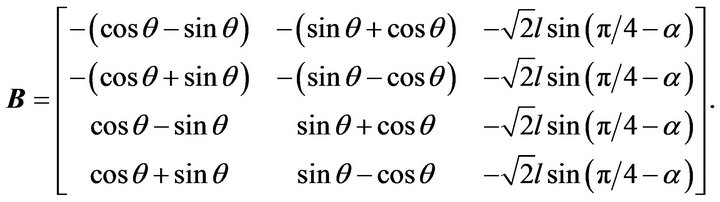
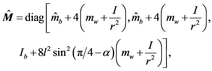
After some straightforward computations, the equations of motion of the mobile robot can be expressed in matrix/vector form as:
 (18)
(18)
where

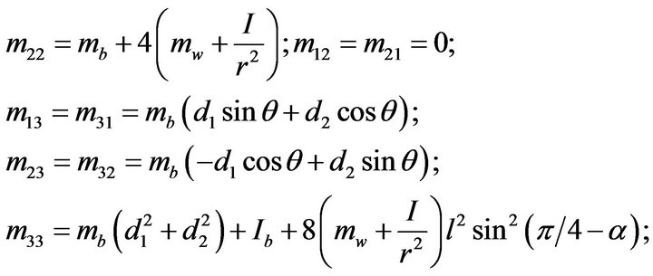
 ;
;
3. Stable Adaptive Control of a Mecanum-Wheeled Robot
3.1. Modeling Uncertainty
In practice, the mass of the platform carrying payload, and the contact friction forces may be varied, thus we can model their uncertainty by letting , and
, and , where
  and
and
 (19)
(19)
are the nominal platform mass and friction vector, respectively. Here is the gravitational constant, and
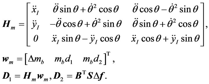
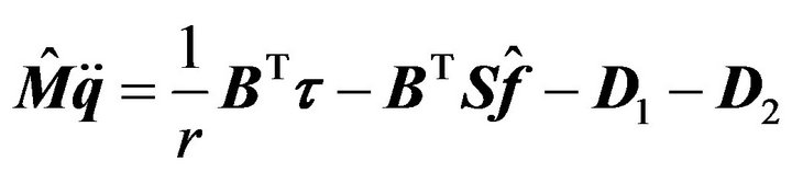
 , are the nominal rolling friction coefficients of the four wheels. Substituting into Equation (18), the dynamics of the mobile robot considering uncertainty can be summarized as follows:
 (20)
(20)
where
3.2. Stable Adaptive Control of a Mecanum-Wheeled Robot
3.2.1. Nominal Control Law Derivation
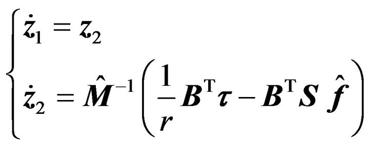
In order to synthesize the adaptive control law, we can first neglect the uncertainty effect, i.e., let  in Equation (20), and consider the following nominal dynamics model:
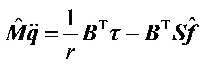 (21)
(21)
Defining the state vector as:
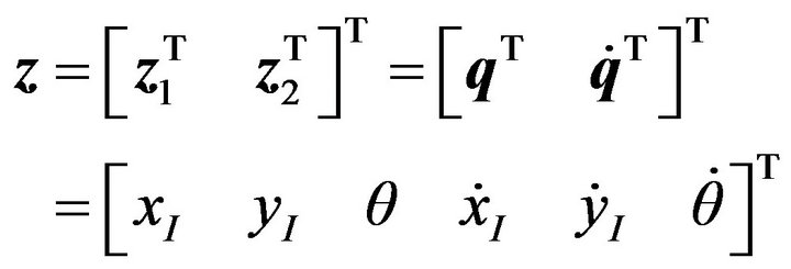
the state equation of the nominal system can be written as
 (22)
(22)
Based on the backstepping method, a stable nonlinear nominal control law can be obtained as follows.
First consider the  subsystem,
  Let
Let
 (23)
(23)
where  is a virtual input. Define the tracking error vector as
 (24)
(24)
where 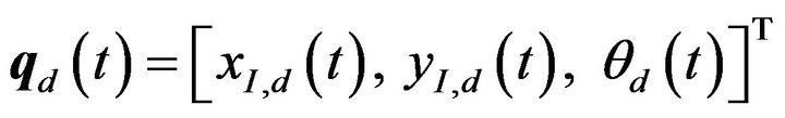 is the desired trajectory vector for the platform. Differentiating Equation (24), we have
 (25)
(25)
Considering the Lyapunov function candidate
 (26)
(26)
where  is symmetric and positive definite, and differentiating Equation (26), we have
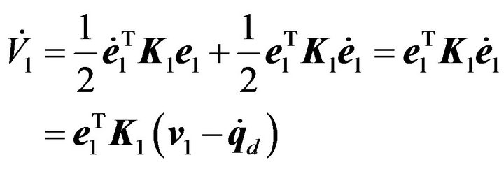 (27)
(27)
Thus, we can choose
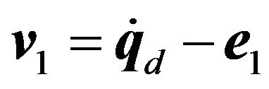 (28)
(28)
and obtain
 (29)
(29)
By Equation (29), we know that  that is, the subsystem is asymptotically stable.
Further, the whole nonlinear system (22) is considered. After introducing new error vector
 (30)
(30)
we can obtain
 (31)
(31)
Then by considering the Lyapunov function candidate as
 (32)
(32)
where is symmetric and positive definite,
 and taking the time derivative of
 , we have
 (33)
(33)
Thus, we can consider the nominal control law as
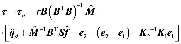 (34)
(34)
and obtain
 (35)
(35)
Since  is negative definite, we know that the equilibrium point
  is exponentially stable.
3.2.2. Adaptive Control of a Mecanum-Wheeled Robot with Uncertainty
Consider the Mecanum-wheeled robot dynamics model with uncertainty :
:
 (20)
(20)
Using the error vectors defined before in the nominal control design,
 (36)
(36)
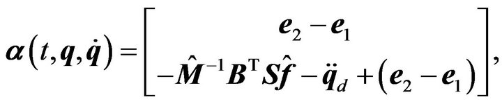
the system’s error dynamics can be obtained by direct differentiating Equation (36) as below:
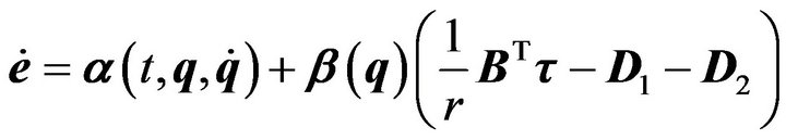 (37)
(37)
where
Consider the following Lyapunov function for adaptive control design,
 (38)
(38)
where  and
and  is a symmetric and positive definite matrix. And taking the time derivative of
 , we have
 (39)
(39)
By the definition of  in Equation (20), we know that it is bounded, i.e.,
  ,
, . Since
  is in linear parametrized form, we can introduce a compensating term
  and choose the control law as
 (40)
(40)
with
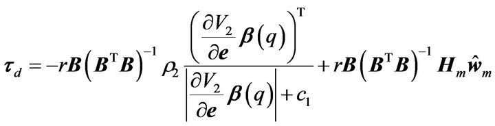 (41)
(41)
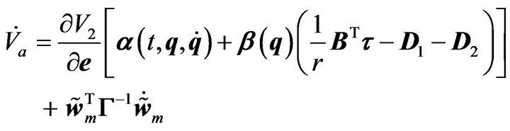
where . Substituting Equations (40) and (41) into Equation (39), we have
 (42)
(42)
Choose the parameter adaptation law as
 (43)
(43)
where  and
and  is the best guess for the unknown parameter vector
 . Since
we have
 (44)
(44)
where
 (45)
(45)
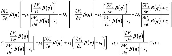
Since  satisfies the following inequality equation [14],
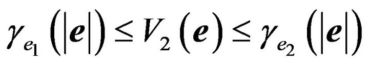 (46)
(46)
where we can choose , thus
 and
and  are class-
 function, and
 , we can obtain
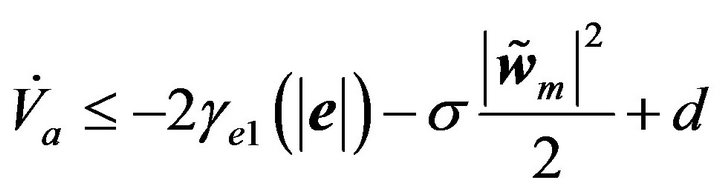 (47)
(47)
Let , then
 , and thus
 . Similarly, while
 , we have
 . Hence, if
  or
or , then
 (48)
(48)
Since
 (49)
(49)
by substituting  and
and  into the right side of Equation (49), we can define
 (50)
(50)
and thus,
Hence, we have
 (51)
(51)
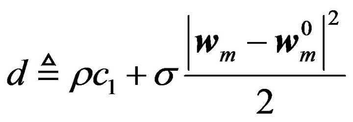
Define
 (52)
(52)
and we thus have .
.
By properly choosing the parameters: 
 constants
  and
and  can be made sufficiently small, and the norm of the tracking error
  is bounded. And thus the adaptive control system is stable.
4. Results and Discussion
In this section, two computer simulation examples are given to illustrate the performance of the proposed adaptive control for the Mecanum-wheeled mobile robot.
The first considers a pure translation along a rectangular desired trajectory in the  plane with fixed orientation
  The platform’s geometric center is planned to move forward from the origin of the inertia frame along
  axis 1 m, then leftward along
  axis 1 m, and then backward along
  axis 1m, and finally move rightward along
  axis 1 m and return to the origin. The desired
  are obtained using the cubic spline method [15] and shown as the dashed lines in Figure 4(a).
The parameters of the mobile robot are selected as follows: mb = 12 kg, I = 0.5 kg·m2, Iw = 4.0378 × 10⁻⁴ kg·m2, a = 0.2 m, b = 0.3 m, l = 0.25 m, mw = 0.313 kg, r = 0.0508 m,  and
and  And the adaptive controller parameters are chosen as:

and

In the simulation, we consider the platform having eccentricity with  and the mass has variation
  The wheels’ contact frictions are assumed with uncertainty
 .
.
The simulation results are shown in Figure 4. Figure 4(a) depicts the tracking performance of the  - and
- and  -axes translation, and the orientation
  variation, and Figure 4(b) shows their tracking errors. We know that the tracking errors along the
  - and
- and  -axes are within ‒0.0063 - 0.0056 m and ‒0.0065 - 0.0062 m, respectively, and the orientation error is within
 . The corresponding control torques of the four Mecanum wheels are shown in Figure 4(c). The adaptation processes of the uncertainty compensation term’s parameters vector
  are shown in Figure 4(d). And the geometric center’s moving trajectory in the
  plane is shown in Figure 4(e).
Considering the same uncertainties as the first case, a second simulation is considered to show the pure rotational control performance. The adaptive control parameters are selected as below:

and
Simulation results of the pure rotation case are shown in Figure 5. Figure 5(a) depicts the tracking performances of the  - and
- and  -axes translation, and the orientation
 , and Figure 5(b) shows their tracking errors. We know that the undesired displacement along the

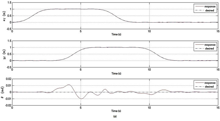

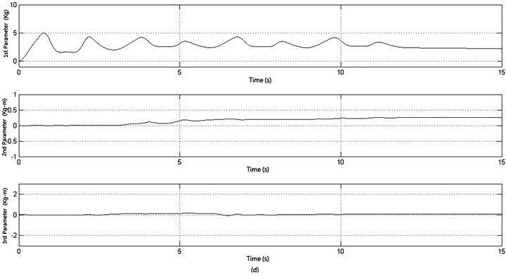
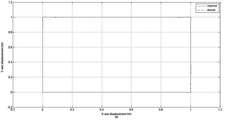
Figure 4. Simulation results of the pure translational case. (a)  and
and  responses; (b) Tracking errors; (c) Control torques,
 ; (d) Compensator parameters adaptation
 ; (e) Tracking results of geometric center,
 .
.
and  -axes can be kept within ‒0.0257 - 0.0235 m and ‒0.0143 - 0.0270 m, respectively, and the orientation
  error is within ‒0.0574 - 0.0362 rad. The corresponding control torques of the four Mecanum wheels are shown in Figure 5(c). The adaptation processes of the uncertainty compensation term’s parameters vector
  are shown in Figure 5(d). And the geometric center’s displacement in
  plane is shown in Figure 5(e).
5. Conclusions
In this paper, Cartesian-space dynamics modeling and stable adaptive control for a four-Mecanum-wheeled robot are considered. Based on the derived 3-DOF dynamics model considering the platform mass variation, eccentricity, and friction uncertainty, a nonlinear stable adaptive control law is derived using the backstepping method via Lyapunov stability theory. A nonlinear damping term is included in the control law to compensate for the estimation error, and the parameters adaptation law with  modification is considered for the uncertainty estimation. Computer simulations are presented to illustrate the control system performance. Real
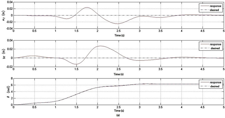
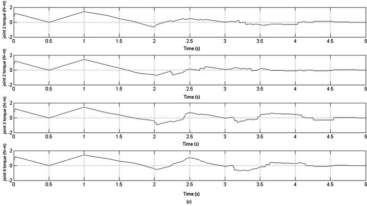
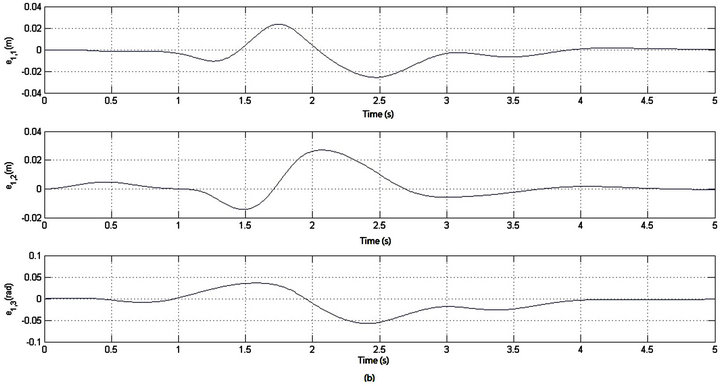


Figure 5. Simulation results of the pure rotational case. (a)  and
and  responses; (b) Tracking errors, (c) Control torques,
 ; (d) Compensator parameters adaptation
 ; (e) Displacement of geometric center
 .
.
implementation study using the suggested control law with microcontroller deserves future consideration.
REFERENCES
- R. Rojas, “A Short History of Omnidirectional Wheels.” http://robocup.mi.fu-berlin.de/buch /shortomni.pdf
- K.-L. Han, H. Kim and J. S. Lee, “The Sources of Position Errors of Omni-Directional Mobile Robot with Mecanum Wheel,” IEEE International Conference on Systems, Man and Cybernetics, 2010, pp. 581-586.
- N. Ould-Khessal, “Design and Implementation of a Robot Soccer Team Based on Omni-directional Wheels,” 2nd Canadian Conference on Computer and Robot Vision, 9-11 May 2005, pp. 544-549. doi:10.1109/CRV.2005.31
- O. Diegel, A. Badve, G. Bright, J. Potgieter and S. Tlale, “Improved Mecanum Wheel Design for Omni-Directional Robots,” Proceedings of the Australasian Conference on Robotics and Automation, Auckland, 2002, pp. 117-121.
- H. Asama, M. Sato, L. Bogoni, H. Kaetsu, A. Matsumoto and I. Endo, “Development of an Omni-Directional Mobile Robot with 3 DOF Decoupling Drive Mechanism,” IEEE International Conference on Robotics and Automation, Nagoya, 1995, pp. 1925-1930.
- R. Siegwart, I. R. Nourbakhsh and D. Scaramuzza, “Introduction to Autonomous Mobile Robots,” 2nd Edition, MIT Press, London, 2011.
- C.-C. Tsai, F.-C. Tai and Y.-R. Lee, “Motion Controller Design and Embedded Realization for Mecanum Wheeled Omni-Directional Robots,” Proceedings of the 8th World Congress on Intelligent Control and Automation, Taiwan, 2011, pp. 546-551.
- N. Tlale and M. de Villiers, “Kinematics and Dynamics Modeling of a Mecanum Wheeled Mobile Platform,” 15th International Conference on Mechatronics and Machine Vision in Practice, Auckland, 2-4 December 2008, pp. 657-662. doi:10.1109/MMVIP.2008.4749608
- P. Viboonchaicheep, A. Shimada and Y. Kosaka, “Position Rectification Control for Mecanum Wheeled OmniDirectional Vehicles,” 29th Annual Conference of the IEEE Industrial Electronics Society, Vol. 1, 2003, pp. 854-859.
- K.-L. Han, O.-K. Choi, J. Kim, H. Kim and J. S. Lee, “Design and Control of Mobile Robot with MecanumWheel,” ICROS-SICE International Joint Conference, Fakuoka International Congress Center, Japan, 2009, pp. 2932-2937.
- J. Park, S. Kim, J. Kim and S. Kim, “Driving Control of Mobile Robot with Mecanum Wheel Using Fuzzy Inference System,” International Conference on Control, Automation and Systems, Gyeonggi-do, 2010, pp. 2519-2523.
- C.-C. Tsai and H.-L. Wu, “Nonsingular Terminal Sliding Control Using Fuzzy Wavelet Networks for MecanumWheeled Omni-Directional Vehicles,” IEEE International Conference on Fuzzy Systems, 2010, pp. 1-6.
- M. W. Spong, S. Hutchinson and M. Vidyasagar, “Robot Modeling and Control,” Wiley, New York, 2006.
- J. T. Spooner, M. Maggiore, R. Ordóñez and K. M. Passino, “Stable Adaptive Control and Estimation for Nonlinear Systems: Neural and Fuzzy Approximator Techniques,” Wiley, New York, 2002. doi:10.1002/0471221139
- C. K. Gau, “Design, Gait Generation and Embedded Microcontroller-Based Single-Axis Servo Controller Implementation for a Biped Walking Robot,” Master Thesis, National Chung Hsing University, Taichung, 2007.