ABSTRACT

A new mathematical system applicable to whatever Brownian problems where the Fickian diffusion equation (F-equation) is applicable was established. The F-equation, which is a parabolic type partial differential equation in the evolution equation, has ever been used for linear diffusion problems in the time-space (t, x, y, z). In the parabolic space (xt^–0.5, yt^–0.5, zt^–0.5), the present study reveals that the F-equation becomes an ellipse type Poisson equation and furthermore the elegant analytical solutions are possible. Applying the new system to one-dimension nonlinear interdiffusion problems, the solutions were previously obtained as the analytical expressions. The obtained solutions were also elegant in accordance with the experimental results. In the present study, nonlinear diffusion problems are discussed in the two and three dimensional cases. The Brownian problem is widely relevant not only to material science but also to other various science fields. Hereafter, the new mathematical system will be thus extremely useful for the analysis of the Brownian problem in various science fields.

1. Introduction

Einstein theoretically revealed that Brownian particles randomly move in accordance with the parabolic law [1]. After then, it was experimentally confirmed by Perrin [2]. The Brownian problem is, however, relevant not only to the motion of particles in material science but also to complex-system science such as life science, computerinformation science, and/or social science [3-6]. Therefore, the Brownian problem is widely relevant to various science fields and is one of the most well-known study subjects in science. In the present study, applying a new mathematical system to diffusion problems, its utility is confirmed through solving them by concrete calculations. The mathematical system used here is also widely applicable to various science fields.

The Fickian diffusion equation (F-equation), which is a continuous equation valid in a conservation system under the condition of no sink and source, is one of the basic equations in physics [7]. When the concentration dependence of the diffusivity and the existence of sink/ source are negligible in diffusion phenomena, the Fequation is a parabolic type linear partial differential equation in the evolution equation. The motion of Brownian particles has been expressed by the F-equation in the time-space, although the F-equation is not directly relevant to the parabolic law. When the diffusevity depends on the concentration in, the diffusivity becomes a function of the independent variables via the concentration. Therefore, even if the F-equation depends only on, the mathematical solutions are impossible as far as another relation between the diffusivity and the concentration is not given. Even if such another relation is given, the mathematical solutions of the nonlinear partial differential equation are almost impossible.

Using the variable transformation of and for the F-equation of, Boltzmann obtained an ordinary differential equation (B-equation) of in 1894 [8]. The variable transformation is physically reasonable in relation to Refs. [1,2]. However, the Bequation has not yet been solved, since another relation mentioned above has not been devised. Then, Matano obtained a diffusivity profile by using a concentration profile of the interdiffusion experimentation between solid metals for the B-equation in 1933 [9]. The empirical method has been widely used for the analysis of the interdiffusion experimentation in metallurgy as an only method to investigate the diffusivity profile. However, the mathematical solutions were not obtained yet.

Recently, the author established a new mathematical system to solve Brownian problems in the parabolic space, where and [10]. Then, two new equations I and II, which correspond to the Fickian first and second laws, were derived as a mathematical system in the parabolic space. The new equation I is an integro-differential equation relevant to the diffusion flux in. Applying it to linear diffusion problems in the one-dimension space, the well-known solutions were obtained by the extremely simple calculations, compared with the previous ones. Further, the elegant analytical solutions of nonlinear diffusion problems were, for the first time, obtained in accordance with the experimental results. However, is not applicable to those problems, since we cannot obtain it as a function of. In this meaning, the new equation I is completely different from the Fickian first law.

In the present study, two and three dimensional problems of the Brownian motion are solved using the new equation II. For linear diffusion problems, the F-equation of becomes an ellipse type Poisson equation of. Based on the mathematical theory, the solution of the Poisson equation is obtained as a linear combination of a particular solution and a complementary function. The present study reveals that the particular solution is easily possible and the complementary function is a constant value to satisfy the given initial and boundary conditions. As a result, the solution is obtained as a linear combination of the well-known error functions. The new mathematical system in the parabolic space yields such elegant solution, compared with the previous one. Further, nonlinear diffusion problems were approximately investigated through the present analytical procedure of the linear problems. As a result, the concentration profile of two and three dimensional nonlinear problems was approximately obtained as an analytical expression, using the previously obtained solution of the one-dimension nonlinear problems.

The new mathematical system applicable to whatever problems where the F-equation is applicable was established. From the concrete calculations of the new mathematical system, it was confirmed that the new mathematical system in the parabolic space is superior in mathematical analysis to the previous one in the ordinary time-space. The analytical solutions obtained here are not only physically reasonable but also mathematically elegant expressions. Hereafter, the new basic equations I and II will be more and more useful for analyzing Brownian problems. For the linear diffusion problems, the present mathematical analysis and that of Ref. [10] are exceedingly simple and elegant in calculation, compared with that of the previous integral transformation of Laplace or Fourier and/or the previous variable-separation method. From the educational point of view, therefore, the new basic equations may take the place of the Fequation in the ordinary text description.

2. New Basic Equations

We summarize the new basic equations derived in the previous study [10]. The Fickian first law is defined as

(1)

in the time-space, where, and are the diffusion flux, the concentration and the diffusivity, using the Dirac’s bracket representation. Applying the divergence theorem to the vector quantity, the F-equation is obtained as

(2)

where the material conversation law is valid under the condition of no sink and source. Boltzmann transformed the equation of

(3)

into the ordinary differential equation of

(4)

where, and because of the initial condition [8].

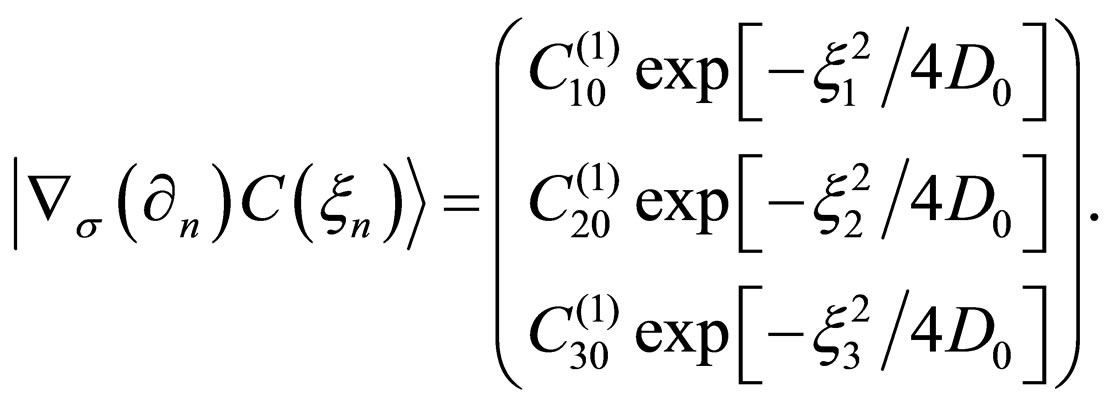
The physical meaning of (4) is not apparent. Then, the author derived the new basic equation I relevant to the diffusion flux in yielding

(5)

Equation (5) corresponds to (1) and the physical meaning is thus apparent. Further, (5) satisfies the conservation law, since it is derived from the F-equation in the conservation system. Here, used in (5) and the notations used in the following are defined as follows.

In the n-dimension parabolic space for n = 1, 2, 3, the nabla vector, the concentration, the diffusivity and the diffusion flux are defined as

For example, they are for,

for and

for using. The diffusivity D means a constant value D = D₀ for and for.

The element of is expressed as

for (6)

where.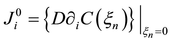

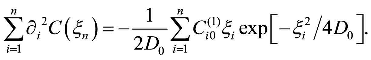
Applying the divergence theorem in the parabolic space to (5), the new basic equation II is obtained as

(7)

and it corresponds to (2). In general, further the following relation of

, (8)

must be mathematically valid between.

Hereinbefore, the mathematical system of (5), (7) and (8) applicable to whatever Brownian problems where the F-equation is applicable was established. It will be revealed in the following that the new mathematical system yields the elegant solutions.

3. Linear Diffusion Problems

In the case of, (6) is rewritten as

for.

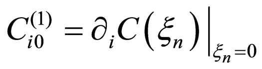Using this equation for, (5) yields

(9)

If we multiply (9) by, the diffusion flux representation is given. Then, (7) becomes the Poisson equation given by

(10)

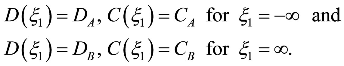
The diffusion problems are solved using the ellipse type differential Equation (10) under the initial and boundary conditions in the following. The initial and boundary conditions of are expressed as:

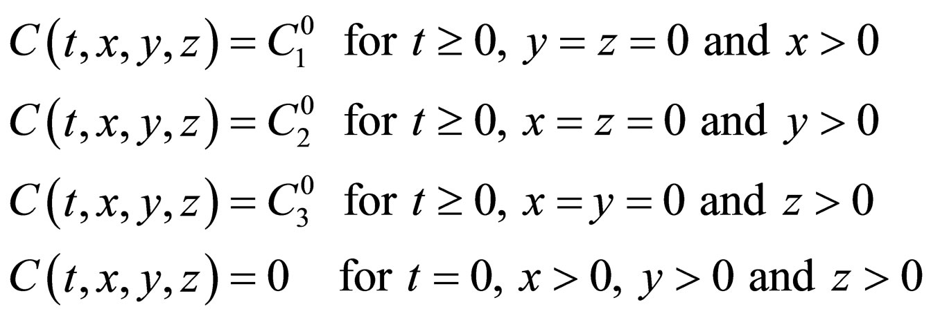
in the time-space and these correspond to

,

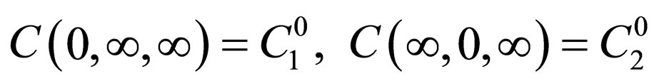
in the parabolic space. In the same manner, those of for the two-dimension space and for the one-dimension space are

and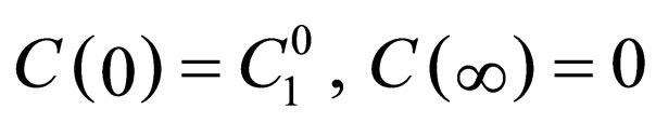

in the parabolic space, respectively.

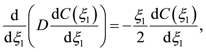
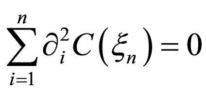
In the analysis of (10), it is easily found that the equation of

(11)

satisfies (10). In other words, (11) is the particular solution of (10). When the solution 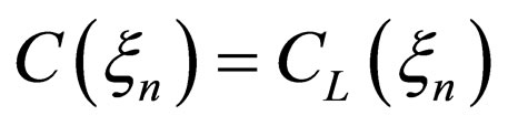of the Laplace equation given by

(12)

satisfies the initial and boundary conditions, the solution of (10) is obtained as

(13)

in accordance with the mathematical theory.

Assuming the equation of

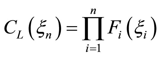(14)

and using the variable-separation method, the solution of (12) is possible. Substituting (14) into (12), the relation of

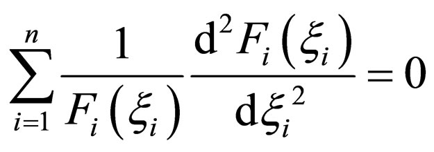
is valid. In order to satisfy this equation for an arbitrary, the equation of

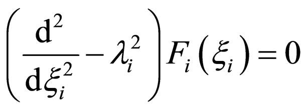(15)

must be valid under the condition of

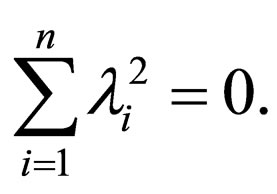(16)

Equation (16) yields for and solution of (15) is expressed as

where are arbitrary constants. In accordance with the present initial and boundary conditions,are obtained. Therefore, the well-known solution is obtained as

(17)

Further, the solutions under other initial conditions are also shown in Ref. [10].

Then, for and, substituting the solution of (15) given by

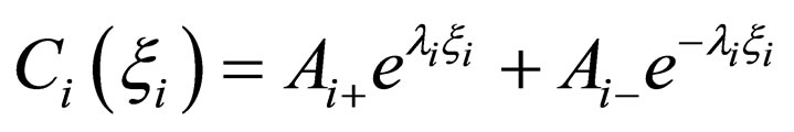
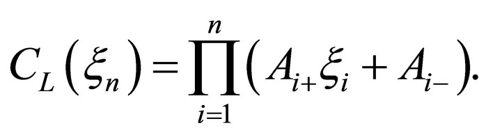
into (14), the general solution of (12) is obtained as

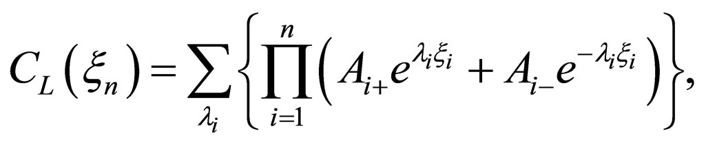(18)

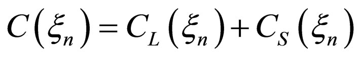
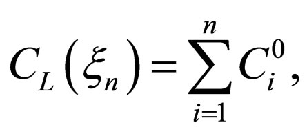
where are arbitrary constants. However, there is no solution to satisfy the initial and boundary conditions. As a result, under the condition of , the general solution of (12) is obtained as

(19)

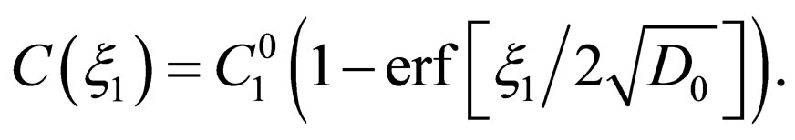
The initial and boundary conditions give. Therefore, the present solution of (12) is obtained as

where 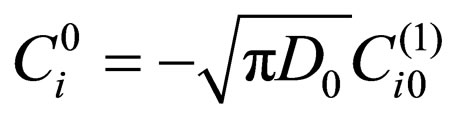in accordance with the initial and boundary conditions.

The solution of (10) is thus obtained as

for (20a)

and/or using for,

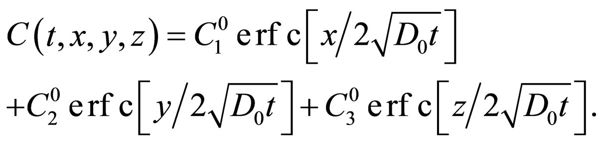(20b)

As described above, the parabolic type F-equation becomes the ellipse type Poisson equation in the parabolic space. As a result, it was apparent that the diffusion behavior is incorporated into the inhomogeneous term of the ellipse type partial differential equation, and that the homogeneous partial differential equation plays a role only to determine the initial and boundary values. As shown in (20a) or (20b), the solution is expressed as the linear combination of the terms resulting from each component of the diffusion flux. The present solution is thus exceedingly simple and elegant, compared with the usual solution of

(21)

where.

From the historical point of view, the diffusion problems have not ever been investigated in the parabolic space for such a long time. In the present study, however, it was revealed that the present analysis of Brownian problems in the parabolic space is exceedingly superior in mathematical calculations to the previous one in the ordinary time-space.

4. Nonlinear Diffusion Problems

The mathematical system for the one-dimension case of (5) and (8) given by

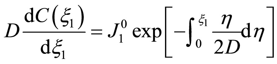(22)

and

(23)

is applicable to the interdiffusion problems between metal plates. In order to discuss two and three dimensional problems, we summarize the results obtained in the previous work [10].

Using the effective diffusivity as an approximation, the solutions of (22) and (23) were obtained as

(24)

and

(25)

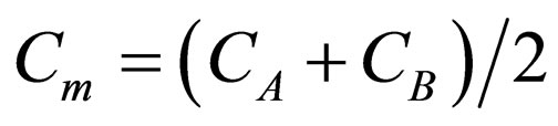
under the initial condition of

Here, the used notations are as follows.

, ,

,

, , ,

,

and is the arithmetical mean of for or the geometrical mean of

for.

Here, if we set in (24) and (25), it is remarkable that (25) becomes the solution when the diffusivity does not depend on the concentration, i.e.,. In other words, (24) and (25) are the generalized solutions regardless of the concentration dependence of the diffusivity.

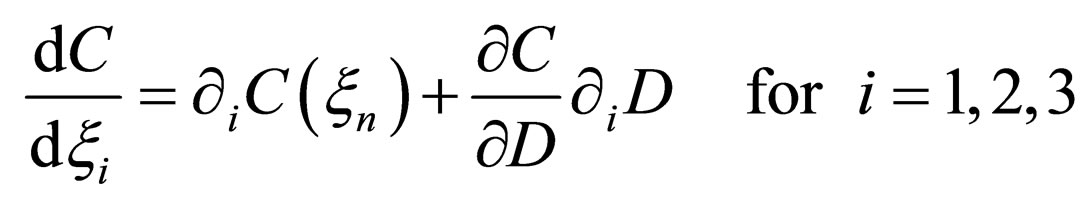
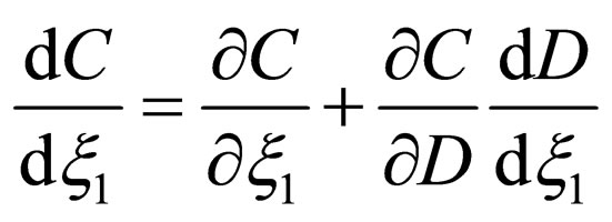
It is extremely difficult to solve the two or three dimensional nonlinear diffusion problems, even if it is approximate. Then, we rewrite (7) into

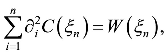(26)

where

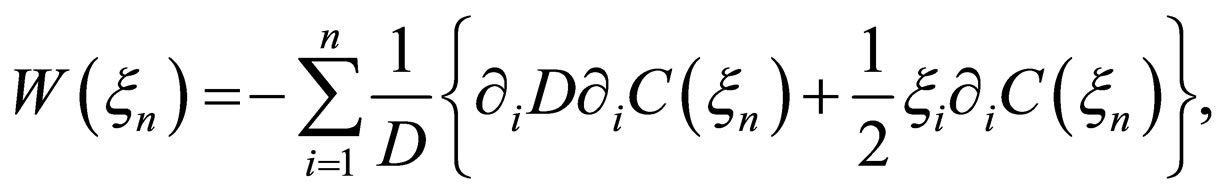(27)

The exact analysis of (26) is impossible, since are included in the right-hand side of (27).

Using the effective diffusivity, physically and mathematically reasonable solutions of (24) and (25) were obtained in Ref. [10]. Then, if we accept the effective diffusivity of in (27) as an approximation, (26) is rewritten as

(28)

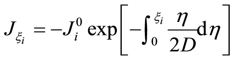
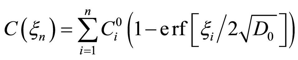
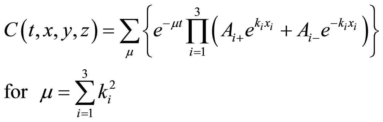
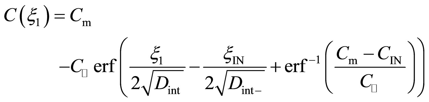
In accordance with the theory of the previous section, the solution of (28) is obtained as

(29)

where are the integral constants to be determined by the initial and boundary conditions. In order to estimate the validity of the solution of (29), it is necessary to compare it with the experimental concentration profile.

5. Conclusions and Discussion

The mathematical system to solve the diffusion problems in the parabolic space was established. The elegant solutions of Brownian problems were obtained in the present study. As a result, it was found that the new basic Equation (5) is exceedingly useful for analyzing Brownian problems.

For the linear Brownian problems, it was found that the diffusion equation becomes the ellipse type partial differential equation in the parabolic space. Further, the diffusion behavior is incorporated into the inhomogeneous term of the ellipse type partial differential equation and the homogeneous differential equation plays a role only to determine the initial and boundary values. We can thus obtain the elegant solutions of Brownian problems.

For nonlinear Brownian problems, it was already confirmed in the previous work that the elegant one-dimension solutions are obtained as the analytical expressions in accordance with the experimental results [10]. In the present study, the concentration profile of the two or three dimensional case was also obtained as the analytical expression of (29) in accordance with the analytical method of the linear problems. It is, however, necessary to investigate the validity between the obtained solutions and the experimental concentration profile. Hereafter, the present mathematical system will be exceedingly useful for the Brownian problem in various science fields.

REFERENCES

- A. Einstein, “Die von der Molekularkinetischen Theorie der Warme Geforderte Bewegung von in Ruhenden Flussiigkeiten Suspendierten Teilchen,” Annalen der Physik, Vol. 18, No. 8, 1905, pp. 549-560. doi:10.1002/andp.19053220806
- J. Perrin, “Mouvement Brownien et Réalité Moléculaire,” Annales de Chimie et de Physique, Vol. 18, No. 8, 1909, pp. 5-114.
- I. Minoura, E. Katayama, K. Sekimoto and E. Muto, “One-Dimensional Brownian Motion of Charged Nanoparticles along Microtubules: A Model System for Weak Binding Interactions,” Biophysical Journal, Vol. 98, No. 8, 2010, pp. 1589-1597. doi:10.1016/j.bpj.2009.12.4323
- C. C. Chen, J. Daponte and M. Fox, “Fractal Feature Analysis and Classification in Medical Imaging,” IEEE Transactions on Medical Imaging, Vol. 8, No. 1, 1989, pp. 133-142. doi:10.1109/42.24861
- K. Arakawa and E. Krotkov, “Modeling of Natural Terrain Based on Fractal Geometry,” Systems and Computors in Japan, Vol. 25, No. 11, 1994, pp. 99-113. doi:10.1002/scj.4690251110
- L. M. Wein, “Brownian Networks with Discretionary Routing,” Operations Research, Vol. 39, No. 2, 1990, pp. 322- 340. doi:10.1287/opre.39.2.322
- A. Fick, “On Liquid Diffusion,” Philosophical Magazine, Vol. 4, No. 10, 1855, pp. 30-39.
- L. Boltzmann, “Zur Integration der Diffusionsgleichung bei Variabeln Diffusionscoefficienten,” Annual Review Physical Chemistry, Vol. 53, No. 2, 1894, pp. 959-964.
- C. Matano, “On the Relation between Diffusion-Coefficients and Concentrations of Solid Metals,” Japanese Journal of Physics, Vol. 8, No. 8, 1933, pp. 109-113.
- T. Okino, “New Mathematical Solution for Analyzing Interdiffusion Problems,” Materials Transactions, Vol. 52, No. 12, 2011, pp. 2220-2227. doi:10.2320/matertrans.M2011137