Applied Mathematics
Vol.5 No.8(2014), Article ID:45617,17 pages DOI:10.4236/am.2014.58108
The Application of Time Series Modelling and Monte Carlo Simulation: Forecasting Volatile Inventory Requirements
Robert Davies, Tim Coole, David Osipyw
Faculty of Design Media and Management, Buckinghamshire New University, High Wycombe, UK
Email: rdavie01@bucks.ac.uk
Copyright © 2014 by authors and Scientific Research Publishing Inc.
This work is licensed under the Creative Commons Attribution International License (CC BY).
http://creativecommons.org/licenses/by/4.0/


Received 8 January 2014; revised 8 February 2014; accepted 15 February 2014
ABSTRACT
During the assembly of internal combustion engines, the specific size of crankshaft shell bearing is not known until the crankshaft is fitted to the engine block. Though the build requirements for the engine are consistent, the consumption profile of the different size shell bearings can follow a highly volatile trajectory due to minor variation in the dimensions of the crankshaft and engine block. The paper assesses the suitability of time series models including ARIMA and exponential smoothing as an appropriate method to forecast future requirements. Additionally, a Monte Carlo method is applied through building a VBA simulation tool in Microsoft Excel and comparing the output to the time series forecasts.
Keywords:Forecasting, Time Series Analysis, Monte Carlo Simulation

1. Introduction
Inventory control is an essential element within the discipline of operations management and serves to ensure sufficient parts and raw materials are available for immediate production needs while minimising the overall stock holding at the point of production and throughout the supply chain. Methodologies including Materials Requirements Planning and Just-in-Time Manufacturing have evolved to manage the complexities of supply management supported by an extensive academic literature. Similarly extensive study into the inventory profiles for spare part and service demand has also been prevalent over the last 50 years.
This paper presents a study of an inventory process that does not fit into the standard inventory models within conventional operations management or for service and spare parts management. In high volume internal combustion engine manufacturing, the demand profile for crankshaft shell bearings follows a highly variable demand profile though there is consistent demand for the engines. The paper reviews the application of both time series analysis and a Monte Carlo simulation method to construct a robust forecast for the shell usage consumption. Section 2 presents the problem statement. Time series analysis is reviewed in Section 3. The Monte Carlo simulation method written in Microsoft Excel VBA is presented in Section 4. Forecasts generated by both the time series models and the simulation are assessed in Section 5 and concluding remarks are presented in Section 6. The analysis utilises usage data provided by a volume engine manufacturer over a 109-week production build period.
2. Problem Statement
The construction of petrol and diesel engines involve fitting a crankshaft into an engine block and attaching piston connecting rods to the crankshaft crank pins [1] . The pistons via the connecting rods turn the crankshaft during the power stroke of the engine cycle to impart motion. Shell bearings are fitted between the crank journals and crank pins and the engine block and connecting rods. During engine operation a thin film of oil under pressure separates the bearing surface from the crankshaft journals and pins. For the smooth operation of the engine, the thickness of the oil film has to be consistent for each crank journal and pin. Though the crankshaft, connecting rods and engine block are machined to exceptionally tight tolerances minor deviations in the dimensions of the machined surfaces mean that the thickness of the oil film will not be consistent across the individual crank journals and pins.
To overcome the problem, the engine designer specifies a range of tolerance bands within an overall tolerance for the nominal thickness of the shell bearing. Similar tolerance bands are specified for the machined surfaces of the engine block and crankshaft. A shell bearing whose thickness is defined within a specific tolerance band is identified by a small colour mark applied during the shell manufacturing process. The engine designer creates a “Fitting Matrix”, where the combination of the tolerance bands for the engine block and crankshaft are compared against which the appropriate shell bearing can be selected. During the engine assembly, the selection process is automated. Embossed marks on the crankshaft and engine block specify the tolerance bands of each machined surface. The marks are either optically scanned or fed into a device that creates a visual display of the colours of the shells to select for assembly. Selection is rapid and does not impede the speed of engine assembly. Table 1 illustrates the set of tolerance bands and associated “Fitting Matrix” for the selection of main bearing shells for a typical engine.
Over time the usage profile for some shells thicknesses can show considerable variation against a consistent demand for the engine itself. The high variation poses a difficult procurement problem for engine assemblers that support high volume automotive production. It is difficult to determine what the usage consumption for high usage shells will be over a future time horizon as the shell bearings can be globally sourced and can require lead times of between 3 and 6 months.
Figure 1 illustrates the consumption trajectory of journal shell sizes over a 109-week sample period that has high demand profiles. The shells are identified by the colour green and yellow. The green shell consumption is highly volatile with sporadic spikes in demand. The yellow shell consumption after showing a rapid decline over

Figure 1. Time series trajectories for green and yellow shell consumption.

Table 1. Bearing selection-fitting matrix.
the first 30 weeks of the sample period settles to lower and less volatile demand than the green shell.
3. Time Series Analysis
Succinctly, a time series is a record of the observed values of a process or phenomena taken sequentially over time. The observed values are random in nature rather than deterministic where the random behaviour is more suitable to model through the laws of probability. Systems or processes that are non-deterministic in nature are referred to as stochastic where the observed values are modelled as a sequence of random variables. Formally:
A stochastic process  is a collection of random variables where T is an index set for which all the random variables
 ,
, ![]() , are defined on the same sample space. When the index set T represents time, the stochastic process is referred to as a time series [2] .
, are defined on the same sample space. When the index set T represents time, the stochastic process is referred to as a time series [2] .
While time series analysis has extensive application, the purpose of the analysis is two-fold [3] . Firstly to understand or model the random (stochastic) mechanism that gives rise to an observed series and secondly to predict or forecast the future values of a series based on the history of that series and, possibly, other related series or factors.
Time series are generally classified as either stationary or non stationary. Simplistically, stationary time series process exhibit invariant properties over time with respect to the mean and variance of the series. Conversely, for non stationary time series the mean, variance or both will change over the trajectory of the time series. Stationary time series have the advantage of representation by analytical models against which forecasts can be produced. Non stationary models through a process of differencing can be reduced to a stationary time series and are so open to analysis applied to stationary processes [4] .
An additional method of time series analysis is provided by smoothing the series. Smoothing methods estimate the underlying process signal through creating a smoothed value that is the average of the current plus past observations.
3.1. Analysis of Stationary and Non-Stationary Time Series
Stationary time series are classified as having time invariant properties over the trajectory of the time series. It is these time invariant properties that are stationary while the time series itself appears to fluctuating in a random manner. Formally, an observed time series  is weakly stationary if the following properties hold:
1) 
2) 
3) 
Further, the time series is defined as strictly stationary if in addition to Properties 1-3, if subsequently:
4) The joint distribution of  is identical to
  for any
 .
.
Conversely, a non-stationary time series will fail to meet either or both the conditions of Properties 1 and 2.
Property 3 states that the covariance of lagged values of the time series is dependent on the lag and not time. Subsequently the autocorrelation coefficient ![]() at lag k is also time invariant and is given by
at lag k is also time invariant and is given by
 (1)
(1)
The set of all![]() ,
,  forms the Autocorrelation Function or ACF. The ACF is presented as a graphical plot. Figure 2 provides an example of a stationary time series with the associated ACF diagram. Successive observations of a stationary time series should show little or no correlation and is reflected in the ACF plot showing a rapid decline to zero.
Conversely, the ACF of a non stationary process will show a gentler decline to zero. Figure 3 replicates the ACF for a non-stationary random walk process.
Stationary time series models are well defined throughout the time series literature where a full treatment of their structure can be found. Representative references include [5] -[8] .
A consistent view of a time series is that of a process consisting of two components a signal and noise. The signal is effectively a pattern generated by the dynamics of the underlying process generating the time series. The noise is anything that perturbs the signal away from its true trajectory [7] . If the noise results in a time series that consists of uncorrelated observations with a constant variance, the time series is defined as a white noise process. Stationary time models are always white noise processes where the noise is represented by a sequence of error or shock terms  where
where . The time series models applicable to stationary and non stationary time series are listed in Table 2.
From Table 2, it is seen that by setting the p, d, and q parameters to zero as appropriate, the MA(q), AR(p) and ARMA(p, q) processes can be presented as sub processes of the ARIMA(p, d, q) process and is illustrated in the hierarchy presented in Figure 4. The stationary processes can be thought of as ARIMA processes that do not require differencing.
Table 2. Description of time series models.
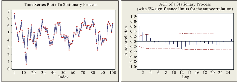
Figure 2. Stationary time series—example ACF.
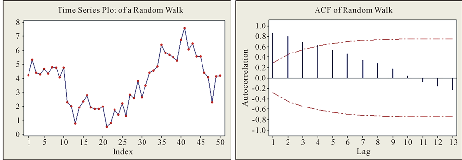
Figure 3. Non-stationary time series example ACF (Random walk).

Figure 4. Time series model hierarchy.
Moreover, the ARIMA process reveals time series models that are not open to analysis by the stationary representations. Two such models are included in Figure 4, the random walk model, ARIMA(0, 1, 0) and the exponential moving average model, ARIMA(0, 1, 1).
Table 3 returns the modelling processes that are applied to stationary and non-stationary time series. The
Table 3. Synthesis of time series models.
equations of the models are replicated in their standard form and in terms of the backshift operator B (see Appendix 1). Time series models expressed in terms of the backshift operator are more compact and enable a representation for the ARIMA process that has no standard form equivalent.
3.2. Model Identification
Initially, inspection of the ACF of a time series is necessary to determine if the series is stationary or will require differencing. There is no analytical method to determine the order of differencing though empirical evidence suggests that generally first order differencing (d = 1) is sufficient and occasionally second order differencing (d = 2) should be enough to achieve a stationary series [7] .
The ACF is also useful to indicate the order of the MA(q) process as it can be shown that for ,
, . Hence the ACF will cut off at lag q for the MA(q) process. The ACF of the AR(p) and ARMA(p, q) processes both exhibit exponential decay and damped sinusoidal patterns. As the form of the ACF’s for these processes is indistinguishable, identification of the process is provided by the Partial Autocorrelation Coefficient (PACF).
The properties of the PACF are discussed extensively in the time series literature and in particular a comprehensive review provided in [9] . Descriptively, the PACF quantifies the correlation between two variables that is not explained by their mutual correlations to other variables of interest. In an autoregressive process, each term is dependent on a linear combination of the preceding terms. In evaluating the autocorrelation coefficient![]() , the term yt is correlated to
, the term yt is correlated to![]() . However, yt is dependent on yt−1 which in turn is dependent on
. However, yt is dependent on yt−1 which in turn is dependent on ![]() and the dependency propagates throughout the time series to
and the dependency propagates throughout the time series to![]() . Consequently, the correlation at the initial lag of the time series propagates throughout the series. The PACF evaluates the correlation between xt is and
. Consequently, the correlation at the initial lag of the time series propagates throughout the series. The PACF evaluates the correlation between xt is and ![]() through removing the propagation effect.
through removing the propagation effect.
The PACF can be calculated for any stationary time series. For an AR(p) process, it can be shown that the PACF cuts off at lag p. The PACF for both the MA(q) and ARMA(p, q) process the PACF is a combination of damped sinusoidal and exponential decay.
The structure of a stationary time series is determined through inspection of both the ACF and PACF diagrams of the series. Table 4 presents the classification of the stationary time behaviour (adapted from [7] [8] ).
Neither the ACF nor PACF yield any useful information with respect to identifying the order of the ARMA (p, q) process. Though there are additional methods that can aid the identification of the required order of the process [7] [8] including the extended sample autocorrelation function (ESACF), the generalised sample partial autocorrelation function (GPACF), and inverse autocorrelation function (IACF) as suitable methods for determining the order of the ARMA model. However, with respect to investigating the structure of a time series both sets of authors agree that with the availability of statistical software packages it is easier to investigate a range of models with various orders to identify the appropriate model and forego the need to apply these additional methods.
The estimation of the parameter coefficients  and
and  can be estimated through Maximum Likelihood Estimation (MLE). An extensive explanation of the MLE application to estimate the parameters of each the models
Table 4. Classification of stationary time series behavior.
listed in Table 2 is provided in [10] . Additionally the parameters of the AR(p) process can be calculated with the Yule Walker Equations [4] [9] .
The robustness of a derived model is assessed through residual analysis of the model. For the ARMA(p, q) process the residual are obtained from
 (2)
(2)
If the residual values exhibit white noise behaviour, the ACF and PACF diagrams of the residual values should not show any discernable pattern then the appropriate model has been chosen and the correct orders of p and q have been correctly identified.
3.3. Generation of Forecasts
Establishing a model that describes the structure of an observed time series enables meaningful forecasts to be drawn from the model. Forecasting methods for each of the models in Table 2 are succinctly described in [11] and are defined as follows:
AR(p) Process:
The forecast for the AR(p) process is based on the property that the expectation of the error terms ![]() are zero. The forecast is developed iteratively from the previous observation to create a one step ahead forecast. The step ahead is denoted by
are zero. The forecast is developed iteratively from the previous observation to create a one step ahead forecast. The step ahead is denoted by


At each successive iteration, the most recent observation drops out of the forecast and replaced by the previous forecast value. At![]() , each term is a forecasted value and continuing the iteration process, the forecast converges onto the mean of the AR(p) process.
, each term is a forecasted value and continuing the iteration process, the forecast converges onto the mean of the AR(p) process.
MA(q) Process:
The expectation of the ![]() terms in the MA(q) process follow a white noise process and so the expectation of all future values of
terms in the MA(q) process follow a white noise process and so the expectation of all future values of![]() , i > 0 is zero. Hence for t > q the forecast of a MA(q) process is just the mean value of the process,
, i > 0 is zero. Hence for t > q the forecast of a MA(q) process is just the mean value of the process,![]() .
.
ARMA(p, q) Process:
The forecast for the ARMA(p, q) process is the combination of the results from the pure AR(p) and MA(q) processes. For t > q, the error terms completely drop out of the forecast.
3.4. Smoothing Methods
Smoothing methods provide a class of time series models that have the effect of reducing the random variation of a time series with the effect of exposing the process signal within the time series. A variety of smoothing models that average the series continually over a moving span of observed values or fit a polynomial approximation to a restricted interval of the series are presented in [12] .
Of the smoothing techniques available, the exponential smoothing model has proved useful due to it’s simplicity of application. First order exponential smoothing is defined by the following recurrence relation:
 (3)
(3)
where ![]() is the smoothing factor
is the smoothing factor .
.
Effectively, first order exponential smoothing is a linear combination of the current observation plus the discounted sum of all previous observations due to the smoothing factor![]() . Moving back through the recursive relation
. Moving back through the recursive relation  geometrically decays and so the older observations have a diminishing contribution to the smoothed estimation of the current value.
Though the recursive relation defined in Equation (3) can be expressed as an ARIMA(0, 1, 1) model, the method was initially developed from first principles in [13] as a means of forecasting inventory.
First order exponential smoothing will for trending data lag behind an increasing trend and lead a decreasing trend. Second order exponential smoothing overcomes this problem as does increasing the value of the smoothing factor [7] . However, providing the time series is showing no systematic trend, first order exponential smoothing is an adequate model to analyse a time series [6] .
The forecast generated from first order exponential smoothing is just the value of the smoothed current value and in principle would extend over all future values. However, as more observed values become available it makes sense to update the forecast.
4. Simulation Application to Evaluate Consumption Rate (Monte Carlo Method)
Frequently in real world scenarios due to the complexity of the system under investigation it may not be possible to evaluate the systems behaviour by applying analytical methods. Under such conditions an alternative approach to model such system is through creating a simulation. Succinctly, simulation methods provide a alternative approach to studying system behaviour through creating an artificial replication or imitation of the real world system [14] . The applications where simulation methods may be useful is extensive and include diverse disciplines such as manufacturing systems, flight simulation, construction, healthcare, military and economics [15] [16] .
Systems or processes that can be modelled through an underlying probability distribution are open to simulation through the Monte Carlo method [17] . The method simulates the behaviour of a system by taking repeated sets of random numbers from the underlying probability distribution of the process under investigation. The development of the method is attributed to the work of Stanislaw Ulam and John von Neumann during the late 1940’s to aid their work in atomic physics for the development of nuclear weapons. Analytical methods were proving difficult if not impossible to apply and Ulam turned to random experimentation to elicit system attributes and behaviour [18] .
A specific application of the Monte Carlo method is dependent on the nature of the underlying probability distribution of the system or process under investigation. However the method application is consistent and will follow the steps outlined in Table 5.
Application of Monte Carlo Method to Shell Consumption Case Study
Visual inspection of the time series trajectories of the shell consumption does not yield an obvious probability distribution so Stage 1 of the Monte Carlo process begins by examining the histograms of the observed series.
Table 5. Monte Carlo method process stages (Adapted from [17] ).
Figure 5 returns the histograms of the consumption of the Green and Yellow Shell consumption for the full trajectory of observed values. The histograms for each shell indicate the data is negatively skewed and so drawing random numbers from a skewed normal distribution for the simulation is deemed appropriate. It can also be shown that the distributions for shorter time spans of the observed values are also skewed.
Stages 2 to 4 of the Monte Carlo process are embedded in a Visual Basic for Applications (VBA) program created in Microsoft Excel to carry out the simulation. Figure 6 provides a schematic of the VBA simulation programme.
The VBA programme incorporates a skewed normal random number generation algorithm developed in [19] that generates random numbers based on the skew value of sample input data. The Excel spreadsheet contains the consumption history for each shell. Upon invoking the simulation, the required sample and forecast periods
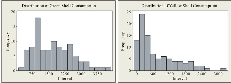
Figure 5. Histograms of green and yellow shell consumption.
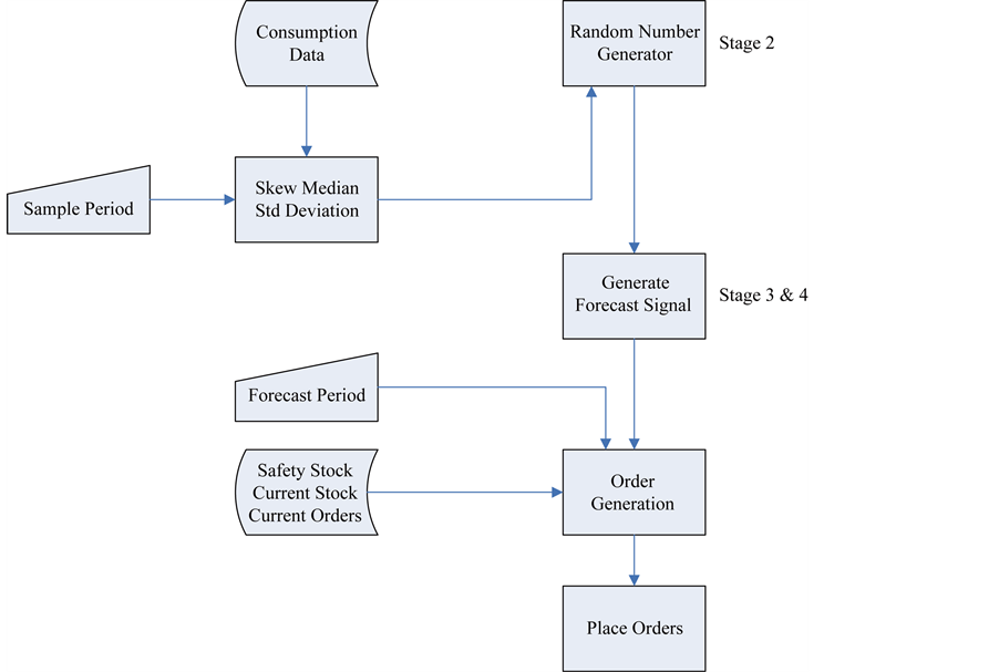
Figure 6. Schematic of VBA simulation programme.
are read from input data in the spreadsheet. For each shell, against the sample period, the skew, median and standard deviation values are calculated and input into the random number generator. For each week of the sample period, the generator calculates 100 positive random numbers to create an average simulated consumption for each week. Since it is impossible to have negative consumption, negative random numbers are rejected. Against each weekly average, an overall average is computed to create the forecast signal.
The random number generator satisfies Stage 2 of Monte Carlo process, while Stages 3 and 4 are satisfied through computation of the forecast signal.
Additional functionality is provided in the simulation tool that over the forecast period will generate orders taking into account current stock levels, safety levels and orders already placed.
5. Generation of Forecasts for the Bearing Shell Consumption
The time series and the Monte Carlo methods described in the preceding sections are applied to the historical shell bearing consumption usage to generate forecasts to create orders to satisfy future engine build requirements. The forecasts of each model are compared to determine if there is either a consistent or significant differences between each method.
5.1. ARIMA (p, d, q)
The purpose of the ARIMA(p, d, q) process is to establish the underlying model that describes the time series through specifying the p and q parameters once the appropriate order of differencing d has identified a stationary process. Model identification is primarily based on inspection of the ACF and PACF diagrams and referencing the Classification Table (Table 4). The robustness of the forecast generated from the identified model is determined by Residual Analysis where primarily if the ACF and PACF diagrams of the residual values show no discernible pattern, the forecast can be assessed as robust [2] -[11] . It is considered that the identification of a time series model requires both judgement and experience and it is recommended that the iterative model building process illustrated in Figure 7 is followed [8] [9] .
The forecasting process is illustrated against the Green Shell consumption replicated in Figure 1. The analysis is carried out using the Minitab® statistical package. The ACF and PACF diagrams are replicated in Figure 8 and with reference to Table 4 indicates that the time series follows an AR(1) process.
Table 6 returns the output generated against 40 observations. The ACF and PACF diagrams of the residual values are returned in Figure 9 and do not show any discernible pattern. The Chi Square statistics appear to be
Table 6. Model estimation for green usage.
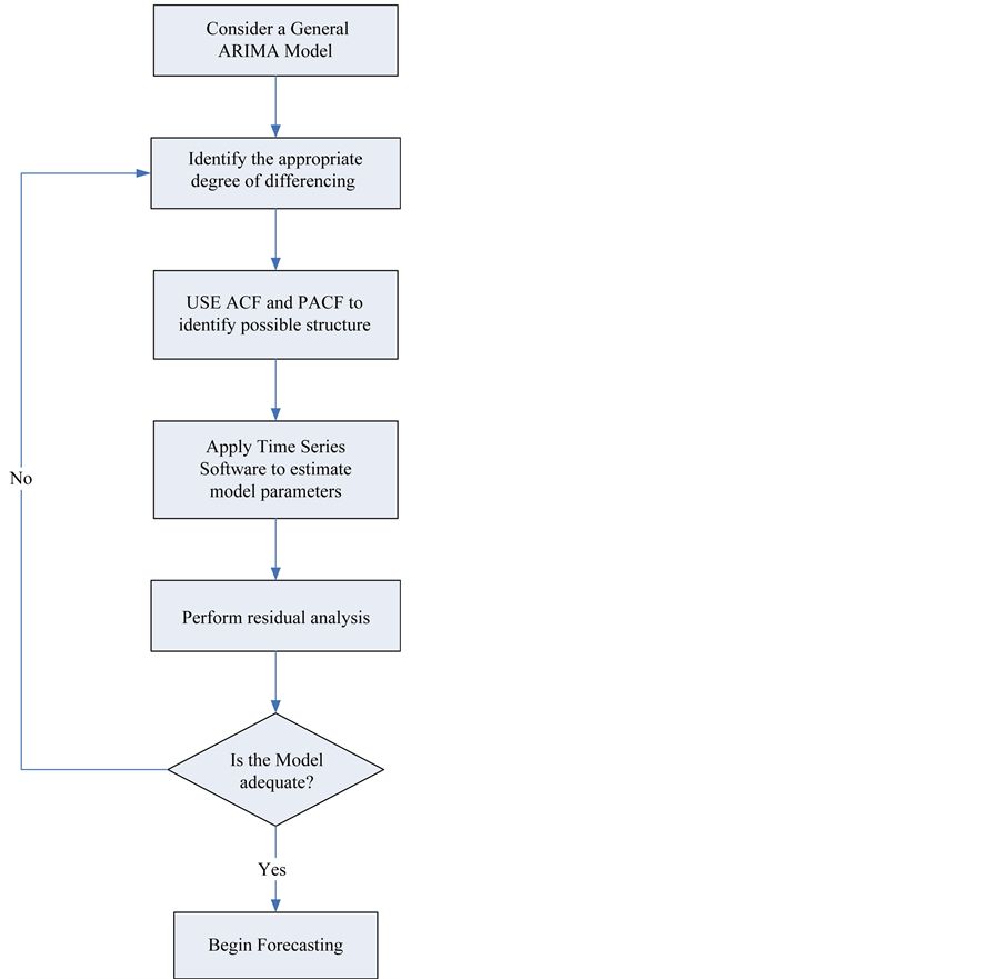
Figure 7. ARIMA model building stages (Adapted from [8] [9] ).

Figure 8. ACF and PACF of green shell usage.
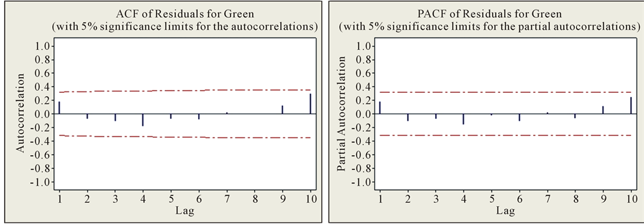
Figure 9. ACF and PACF for residuals of the AR(1) process.
low and diminish as the number of lags increases.
Evidence therefore exists to support that the residuals follow a white noise process and the AR(1) is a robust representation of the observed time series.
The AR(1) process is defined by

The forecast for the process will converge onto the process mean, .
.
The procedure applied to the Yellow shell consumption also resulted in an AR(1) process. Though the details are omitted, the AR(1) process is defined by

The forecast for the process will converge onto the process mean, .
.
5.2. Exponential Smoothing
The application the first order exponential smoothing method requires a choice of smoothing factor ![]() and the number of observations to smooth against. There is no analytical method to determine the optimum choice of smoothing factor and it is necessary to investigate various levels of
and the number of observations to smooth against. There is no analytical method to determine the optimum choice of smoothing factor and it is necessary to investigate various levels of ![]() and choose the smoothing factor that minimises the squared sum of the forecast errors
and choose the smoothing factor that minimises the squared sum of the forecast errors  defined by
 .
.
Similarly there is no method to determine the optimum number of observations to forecast against. The influence of past the observations decays geometrically over time and the impact of the decay can be evaluated against a set of observations.
Table 7 returns generated forecasts for the varying levels of ![]() against both the Green and Yellow shell data where the full set of 109 observations are used. Due to the magnitude of errors, the square root of
against both the Green and Yellow shell data where the full set of 109 observations are used. Due to the magnitude of errors, the square root of  is returned in Table 7.
There is a distinct contrast between the two forecasts. Forecast accuracy for the Green consumption increases as ![]() increases and is a consequence of the volatility of the series. For the Yellow consumption forecast accuracy is assured at
increases and is a consequence of the volatility of the series. For the Yellow consumption forecast accuracy is assured at![]() , where
, where  takes the minimum value. Evident for both time series is that the forecast is influenced by the level of the smoothing factor
![]() . The choice of smoothing factor for the Yellow forecast is defined by the existence of a minimum
. The choice of smoothing factor for the Yellow forecast is defined by the existence of a minimum . The choice of smoothing factor for the Green forecast is not so clear. By inspection of Table 6, choosing
 ![]() would appear appropriate as the forecast reduces at
would appear appropriate as the forecast reduces at ![]() drops slightly.
drops slightly.
Table 8 returns the forecast generated at different observation levels for specific choices of smoothing factor![]() .
.
Variation in the forecast level only becomes apparent at the lower number of observations and the variation is insignificant relative to the level of each forecast and the width of the confidence intervals.
The evidence from Table 7 and Table 8 suggests that the level of smoothing factor is critical with respect to generating a robust forecast while the choice of the number of observations to forecast against is not critical.
5.3. Monte Carlo Simulation
Table 9 returns output from the simulation programme for a range of sample periods for both the Green and Yellow shell consumption. What is clear from both sets of simulations is that for any sample period the simulated forecast signals are consistent. For the Green simulation as the sample period increases, volatility of the consumption is exposed to the simulation. As the sample period increases, the standard deviation increases resulting in an inflated forecast relative to the sample mean. For the Yellow simulation, as the sample period is
Table 7. Forecasts generated against smoothing factor level.
Table 8. Forecasts generated against number of observations.
Table 9. Simulated forecast output.
extended, the standard deviation has not increased significantly reflecting that over extended sample periods the distribution of observations has a greater consistency.
The simulation process is sensitive to excessive volatility resulting in an inflated forecast signal. In principle the affect of the volatility can be overcome by reducing an excessive observation to say within one or two standard deviations of the sample mean. The difficulty in this approach is creating a consistent rule that would apply to all excessive observations. Setting a trigger point at for example 2.5 standard deviations above the sample, an observation at 2.6 standard deviations would be excessively reduced while an observation at 3.5 standard deviations may not be reduced enough.
5.4. Comparison of Forecasting Methods
Table 10 returns the observations of the shell consumption for the following 12 weeks beyond the original observations and the respective graphs of the time series is returned in Figure 10.
A summary of the output from each method is presented in Table 11 where the totals of each forecast are compared to the total of the observed values over the forecast period.
The forecast signals are reasonably close to one another. Though the simulated forecast signal for the Yellow shell is significantly lower than the signals generated by the time series methods, the total forecast is in excess of the observed consumption over the forecast period. The consistency of the forecast signals imply that each modelling processes is robust so indicating the reliability of the signals to generate purchase orders for the shells.
Table 10. Observed shell consumption over forecast period.
Table 11. Summary of forecast output.
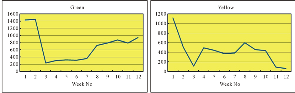
Figure 10. Time series observations over forecast period.
6. Conclusions
Historically, forecasting future demand of the crankshaft shells has proven exceptionally difficult. The purchasing professionals within the case study environment having no experience of applying formal forecasting methods placed orders on the crankshaft shell suppliers that were effectively a “best guess”. To mitigate the need to guess, formal time series analysis was assessed as a suitable approach to modelling demand along with a Monte Carlo simulation method coded in Microsoft Excel VBA.
The forecasts generated by the exponential smoothing and autoregressive process are remarkably close. The simulation process though proving to be sensitive to volatile consumption with judgement of the physical time series, an appropriate forecast signal can be found.
The advantage of the exponential smoothing method lies in its simplicity of execution. The method is open to coding in VBA and would therefore negate the need for specialised software. Though for a volatile time series, it may not be possible to find a smoothing factor that will maximise forecast accuracy. However, choosing a smoothing factor between 0.5 and 0.7 should provide an appropriate forecast signal.
The ARIMA process requires interaction between the user and the modelling process as the ACF and PACF have to be inspected to determine the structure of the model. Though in this study, the autoregressive models were basic AR(1) models, future trajectories may follow more complex ARIMA models. It is recommended that at least 30 observations of a time series are needed to enable the generation of a meaningful forecast. In the current study, there is over two years of data available so the restriction did not apply. However, for the build of a new engine, the application of the ARIMA model would be impeded until there are enough observations to forecast against. Empirical evidence from this study confirms that the exponential smoothing model can produce meaningful forecasts with at least 10 observations and would therefore provide a more robust method of forecasting with limited data sets.
The simulation method provides a seamless process to generate forecast signals and offers additional functionality to generate orders. Execution of the simulation for the complete shell requirement is efficient and completes generally in less than two minutes. The simulation is sensitive to volatile demand and can over inflate the forecast signal.
Monte Carlo methods have proved effective to model a diverse range of complex applications. While the method is consistent, the execution of the method to a specific application has to be tailored to that application. The functionality of the simulation method created within this study is restricted to modelling the forecast consumption of the crankshaft shells. Conversely, the time series methods are universally applicable.
Inspection of Table 11 confirms that for each of methods, the forecast signals are close to each other and so with respect to forecast accuracy there is no one best method. Moreover, since the forecast signals are close to one another, the purchasing professionals are confident that a robust forecast signal is being generated.
Currently, the appropriate choice of forecasting tool is the simulation method as it provides a seamless process not only to generate the forecast signal but also generate the orders. Building a VBA programme around the exponential smoothing process should in principle provide the functionality provided by the simulation method.
Inventory profiles exhibited by the consumption of the crankshaft shells are rare within the discipline of Operations Management. Conventional though rigorous methods of inventory control that include Materials Requirement Planning and Just-in-Time Kanban systems do not apply to the procurement of the crankshaft shells. Moreover, due to the rarity of such inventory profiles, there does not appear to be any significant research into this unique area of inventory management. The application of the Monte Carlo simulation method and time series analysis begins to close this gap.
References
- Hillier, V.A.W. and Coombes, P. (2004) Fundamentals of Motor Vehicle Technology Book 1. 5th Edition, Nelson Thornes Ltd, Cheltenham.
- Woodward, W.A., Gray, H.L. and Elliot, A.C. (2012) Applied Time Series Analysis. CRC Press, Boca Baton.
- Cryer, J.D. and Chan, K.S. (2008) Time Series Analysis: With Applications in R. Springer. Science + Business Media, London.
- Brockwell, P.J. and Davis, R.A. (2010) Introduction to Time Series and Forecasting. 2nd Edition, Springer Texts in Statistics, New York.
- Peña, D., Tiao, G.C. and Tsay, R.S. (2000) A Course in Time Series Analysis. Wiley-Interscience, New York.
- Chatfield, C. (2006) The Analysis of Time Series, an Introduction. 6th Edition, Chapman and Hall, London.
- Montgomery, D.C., Jennings, C.L. and Kulachi, M. (2008) Introduction to Time Series Analysis and Forecasting. WileyBlackwell, New Jersey.
- Bisgard, S. and Kulachi, M. (2011) Time Series Analysis and Forecasting by Example. Wiley & Sons Inc., New York. http://dx.doi.org/10.1002/9781118056943
- Box, G.E.P., Jenkins, G.M. and Reinsel, G.C. (2008) Time Series Analysis. Forecasting and Control. 4th Edition, Wiley & Sons Inc., New Jersey.
- Hamilton, J.D. (1994) Time Series Analysis. Princeton University Press, Princeton.
- Kirchgässner, D., Wolters, J. and Hassler, U. (2013) Introduction to Modern Time Series Analysis. 2nd Edition, Springer Heidelberg, New York. http://dx.doi.org/10.1007/978-3-642-33436-8
- Kendall, M. (1976) Time Series. 2nd Edition, Charles Griffin and Co Ltd., London and High Wycombe.
- Brown, R.G. (1956) Exponential Smoothing for Predicting Demand. http://legacy.library.ucsf.edu/tid/dae94e00
- Robinson, S. (2004) Simulation: The Practice of Model Development and Use. John Wiley and Sons, Chichester.
- Banks, J., Carson, J.S. and Nelson, B.L. (1996) Discrete-Event System Simulation. 2nd Edition, Prentice-Hall, Upper Saddle River.
- Singh, V.P. (2009) System Modelling and Simulation. New Age International Publishers, New Delhi.
- Sokolowski, J.A. (2010) Monte Carlo Simulation. In: Sokolowski, J.A. and Banks, C.M., Eds., Modelling and Simulation Fundamentals: Theoretical Underpinnings and Practical Domains, Wiley & Sons Inc., New Jersey, 131-145. http://dx.doi.org/10.1002/9780470590621.ch5
- Metropolis, N. and Ulam, S. (1949) The Monte Carlo Method. Journal of the American Statistical Association, 44, 335-341. http://www.amstat.org/publications/journals.cfm http://dx.doi.org/10.1080/01621459.1949.10483310
- Azzalini, A. (2008) The Skew-Normal Probability Distribution. http://azzalini.stat.unipd.it/SN/
Appendix 1. Backshift and Differencing Operators
Frequently within the time series literature, time series are presented using difference operator denoted by ![]() and the lag or backshift operator B. Kirchgässner et al. (2013) succinctly define the properties of both operators. The essential properties of the operators are replicated as follows:
and the lag or backshift operator B. Kirchgässner et al. (2013) succinctly define the properties of both operators. The essential properties of the operators are replicated as follows:
First order differencing is expressed using the difference operator ![]() such that
such that
 Second order differencing is expressed as
![]()
The backshift operator B has the effect of “delaying” a time series by one period, such that

Applying the backshift operator to , the following is obtained
![]()
In general
 (A1)
(A1)
Applying property (A1) to a time series of the form

yields a polynomial in B such that

The backshift operator can be related to a first order difference in the following way

Second order differencing

If a series is differenced d times then it can be shown that