Applied Mathematics
Vol.5 No.2(2014), Article ID:42167,22 pages DOI:10.4236/am.2014.52028
Optimal Consumption under Uncertainties: Random Horizon Stochastic Dynamic Roy’s Identity and Slutsky Equation
1Center of Game Theory, St Petersburg State University, St Petersburg, Russia
2SRS Consortium for Advanced Study in Cooperative Dynamic Games, Shue Yan University, Hong Kong, China
Email: dwkyeung@hksyu.edu
Received June 17, 2013; revised July 17, 2013; accepted July 24, 2013
ABSTRACT
This paper extends Slutsky’s classic work on consumer theory to a random horizon stochastic dynamic framework in which the consumer has an inter-temporal planning horizon with uncertainties in future incomes and life span. Utility maximization leading to a set of ordinary wealth-dependent demand functions is performed. A dual problem is set up to derive the wealth compensated demand functions. This represents the first time that wealth-dependent ordinary demand functions and wealth compensated demand functions are obtained under these uncertainties. The corresponding Roy’s identity relationships and a set of random horizon stochastic dynamic Slutsky equations are then derived. The extension incorporates realistic characteristics in consumer theory and advances the conventional microeconomic study on consumption to a more realistic optimal control framework.
Keywords:Optimal Consumption; Uncertain Inter-Temporal Budget; Stochastic Dynamic Programming; Slutsky Equation
1. Introduction
In a ground-breaking analysis by Slutsky [1], the foundation for rigorous analysis of optimal consumption decision was laid. This masterpiece which brought mathematical rigor to demand analysis is undisputedly an integral part of contemporary mainstream economics. It allows the problem of the consumer to be analyzed in terms of a utility maximization problem subject to a budget constraint. A dual problem to the utility maximization problem is the minimization of the budget (income) subject to maintaining the utility level achieved before. In particular, the effect of a price change on the demand of goods can be decomposed into tractable terms from the primal and dual problems yielding significant economic implications. This prominent contribution in consumer theory, known as the Slutsky equation, was christened by John Hicks as the “Fundamental Equation of Value Theory”. An important economic implication of the Slutsky equation is the now famous Hicksian decomposition which separates the effect of a change in price on demand into a pure substitution effect and an income effect. The papers [2-7] propagated Slutsky’s classic work. Yeung [8] extends Slutsky’s work to a dynamic framework in which the consumer has a T-period life span with future incomes being uncertain.
Another milestone in consumer theory is the Roy’s identity [9] which provides an often invoked mathematical result in consumer theory. The identity is also instrumental to prove the Slutsky equation. In this paper, uncertainties in future incomes and the consumer’s life span are incorporated to reflect the realities in consumer choice. In particular, optimal consumption choice under these two types of uncertainties is examined. Intertemporal wealth-dependent ordinary demand functions and wealth compensated demand functions are obtained. Two of the most crucial foundations in consumer theory—Roy’s identity and Slutsky equation—are derived in a random horizon stochastic dynamic framework.
The paper is organized as follows. We first present a model of utility maximization by a consumer with an uncertain life span and an uncertain inter-temporal budget in Section 2. In Section 3, a set of wealth-dependent ordinary demands is characterized. The Roy’s identity in a random horizon stochastic dynamic framework is derived in Section 4. The dual problem is formulated in Section 5 and wealth compensated demand functions are obtained. Stochastic dynamic Slutsky equations for the consumer with an uncertain life span are formulated in Section 6. An illustration with explicit utility functions is given in Section 7. Section 8 concludes the paper.
2. Utility Maximization under Random Life Span and Uncertain Income
Consider the case of a consumer whose life-span involves  periods where
  is a random variable with range
  and corresponding probabilities
 . Conditional upon the reaching of period
 , the probability of the consumer’s life-span would last up to periods
  becomes respectively
 (1)
(1)
We use  to denote the quantities of goods consumed and
  the corresponding prices in period
 . The consumer maximizes his expected inter-temporal utility
 , (2)
, (2)
subject to the budget constraint characterized by the wealth dynamics
 (3)
(3)
where  is the interest rate;
  is the random income that the consumer will receive in period
 ; and
; and , for
, for , is a set of statistically independent random variables, and
  is the expectation operation with respect to the statistics of
 . The random variable
  has a non-negative range
  with corresponding probabilities
 .
.
Again, the time preference factor is embodied in the utility function the random variable  has a value of zero with probability 1 because the consumer will receive no income in period
 . Moreover, under the axiom of non-satiation, the consumer will spend all his wealth in the last period of his life span and therefore
 . The problem (2)-(3) is a discrete-time stochastic control problem (see [10,11]).
Now consider the case when the consumer has lived to period ![]() and his wealth is
and his wealth is . The consumer problem can formulized as the maximization of the payoff:
 , (4)
, (4)
subject to the budget constraint characterized by the wealth dynamics
 (5)
(5)
In a stochastic dynamic framework, strategy space with state-dependent property has to be considered. In particular, a pre-specified class  of mapping
  with the property
 , for
, for , is the strategy space and each of its elements is a admissible strategy. We define the value function
  and the set of strategies
  which provides an optimal consumption solution as follows:
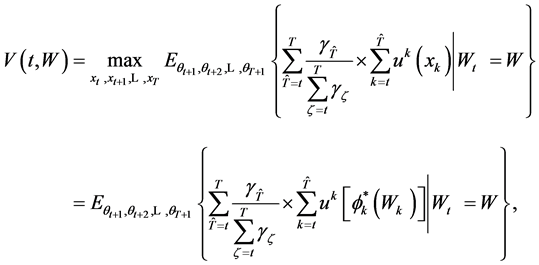 (6)
(6)
for .
.
In particular,  reflects the expected inter-temporal utility that the consumer will obtain from period
 ![]() to the end of his life span. Following the analysis of Yeung and Petrosyan [12,13] one can derive an optimal solution to the random-horizon consumer problem (2)-(3) as follows:
to the end of his life span. Following the analysis of Yeung and Petrosyan [12,13] one can derive an optimal solution to the random-horizon consumer problem (2)-(3) as follows:
Theorem 2.1. A set of consumption strategies  provides an optimal solution to the random horizon consumer problem (2)-(3) if there exist functions
 , for
, for , such that the following recursive relations are satisfied:
 and
and ,
,
 (7)
(7)
Proof. Following Bellman’s [14] technique of dynamic programming we begin with the last period/period. By definition, the utility of the consumer at period  and therefore
 .
.
We first consider the case when the consumer survives in the last period  and the state
 . The problem then becomes
 (8)
(8)
subject to
 . (9)
. (9)
Since  with probability 1,
  and
and , the problem in (8)-(9) can be expressed as the second equation in Theorem 2.1.
Now consider the problem in period . Invoking the probabilities that the consumer can live up to periods
  and
and , the problem in period
  can be expressed as maximizing
 (10)
(10)
subject to
 (11)
(11)
If the value function  exists, the problem (10)-(11) can be expressed as a single period problem:
 (12)
(12)
Now consider the problem in period . Following the analysis above, the problem in period
 ![]() becomes the maximization of the expected payoff
becomes the maximization of the expected payoff
 (13)
(13)
subject to
 (14)
(14)
Note that in (13) the term
 (15)
(15)
gives the expected intertemporal utility to be maximized in period . If the value function
  exists, the problem (13)-(14) can be formulated as a single period problem which maximizes the expected payoff
 (16)
(16)
If  exists, we have the third set of equations in Theorem 2.1. Hence Theorem 2.1 follows. ■
The stochastic optimal state trajectory derived from Theorem 2.1 is characterized by:

We use  to denote the set which contains all possible values of wealth
  at period
  along the optimal trajectory generated by Theorem 2.1.
3. Wealth-Dependent Ordinary Demand under Uncertain Life Span and Income
In this section, we consider the primal problem of deriving wealth-dependent ordinary demand functions in which the consumer maximizes his inter-temporal expected utility subject to uncertain inter-temporal budget and life span. Following the analysis in [8] we first consider the case when the consumer survives in the last period, that is period . Let
. Let  denote the consumer’s wealth in period
 . Given that
  and
and , to exhaust all the wealth in this period,
 . Hence the consumer faces the problem
 (17)
(17)
Problem (17) is a standard single period utility maximization problem. Setting up the corresponding Lagrange problem and performing the relevant maximization one obtains a set of first order conditions. It is well-known (see [15]) that if the set of first order conditions satisfies the implicit function theorem, one can obtain the ordinary demand as explicit functions of the parameters  and
and , that is:
 (18)
(18)
One can readily observe that  corresponds to the optimal consumption strategies
  in Theorem 2.1. Substituting (18) into (17) yields the indirect utility function in period
  as
as
 . Invoking the definition in Equation (6),
  equals the function
 in Theorem 2.1.
Now consider the case when the consumer survives in the second last period . If wealth equals
  in this period, the problem in concern becomes

subject to the inter-temporal budget
 (19)
(19)
Let  denote the wealth at period
  if
if  has occurred.
Using the indirect utility function , the problem facing the consumer in period
  can be expressed as a single-period problem:
 (20)
(20)
First order condition for a maximizing solution yields
 (21)
(21)
Again, with the implicit function holding, (21) can be solved to yield the ordinary demands in period 
as , for
, for . Substituting
  into (20) yields the inter-temporal indirect utility function
 . Invoking Equation (6) and Theorem 2.1,
 corresponds to
 .
.
Repeating the analysis for periods  to 1 yields the consumer problem at period
  as
as
 (22)
(22)
where ,
,  , and
, and  is the short form for the vector
 .
.
First order condition for a maximizing solution to the problems in (22) can be obtained as:
 (23)
(23)
for  and
and .
.
Note also the condition that in period , good
 ![]() will be consumed up the point where marginal utility of consumption
will be consumed up the point where marginal utility of consumption  equals
  times the expected marginal utility of wealth
 .
.
In particular, the expected marginal utility of wealth takes into consideration the random future income and the probability of the consumer surviving in period . Solving (23) yields the ordinary demands in period
  as:
as:
 (24)
(24)
After solving the primal consumer problem which maximizes expected utility subject to an uncertain intertemporal budget and life span, we proceed to derive the Roy’s identity result in a random horizon stochastic dynamic framework.
4. Random Horizon Stochastic Dynamic Roy’s Identity
In this section we derive the random horizon version of the stochastic dynamic Roy’s Identity. Invoking (23) we obtain the identity
 (25)
(25)
Differentiating the inter-temporal indirect utility function in (25) with respect to :
:
 (26)
(26)
where ,
,  and
and .
.
Invoking the first order conditions in (23) the term inside the curly brackets vanishes, condition (26)then becomes:
 (27)
(27)
The effect of a change in initial wealth on the maximized utility can be obtained by differentiating  in (25) with respect to
 :
:
 (28)
(28)
Again, invoking the first order conditions in (23), the term inside the curly brackets vanishes, condition (28) then becomes:
 (29)
(29)
Dividing the right-hand-side of (27) by the right-hand-side of (29) yields:
 (30)
(30)
Condition (30) provides a random horizon stochastic dynamic version of the Roy’s Identity involving a change in current prices.
Then we consider deriving the random horizon stochastic dynamic Roy’s Identity for a change in prices in current and future periods.
Theorem 4.1. Random Horizon Stochastic Dynamic Roy’s Identity
 (31)
(31)
 (32)
(32)
for ,
,  and
and where
where
 (33)
(33)
Proof. See Appendix A of this Chapter. ■
Theorem 4.1 gives the random horizon stochastic dynamic Roy’s identity. Invoking (73) in the proof of Theorem 4.1 in Appendix A, an alternative form of the random horizon stochastic dynamic Roy’s identity can be expressed as:
 (34)
(34)
for ,
, , and
, and .
.
5. Duality and Wealth Compensated Demand
In this section, we invoke the duality principle in consumer theory to construct wealth compensated demand functions under an uncertain inter-temporal budget and a random life span by considering the dual problem of minimizing expenditure covered by the current wealth subject to maintaining the level of utility achieved in the primal problem. Again, following the analysis in [8] we first consider the last period in which  is the consumer’s wealth if he survives in the period. Since wealth equals income in this period, to derive the compensated demand we follow the standard single period consumer problem of

subject to achieving the level of utility
 (35)
(35)
Setting the corresponding Lagrange function and performing the minimization operation yields a set of first order conditions. With the implicit function theorem holding for the first order conditions one can obtain the wealth (income) compensated demand functions as
 (36)
(36)
Substituting (36) into (35) yields the wealth-expenditure function .
.
Now we proceed to period  and let wealth in this period be
 . To obtain the wealth compensated demand function in period
  we consider the problem of minimizing expenditure covered by current wealth in the period to bring about the expected inter-temporal utility
  from the primal problem. However, wealth
  in period
  does not only cover consumption expenditure
  in the period
  but also part of the consumption expenditure in period
 . To delineate expenditures attributed to wealth in period
  we first invoke the dynamical Equation (3) and express
  as:
as:
 . (37)
Using the wealth expenditure function  in period
  and taking expectation over the random variable
  in (37) one can obtain a crucial identity relating wealth to current and expected future expenditures attributable to wealth as:
 (38)
(38)
Using (38) the consumer’s dual problem in period  can be formulated as minimizing wealth expenditure
 (39)
(39)
with respect to  subject to the constraint
 (40)
(40)
Since  is a set of wealth compensated demands that leads to the level of utility
 so
so  equals
 .
.
Invoking 
the constraint (40) can be expressed as:

Setting the Lagrange function and performing the relevant optimization operation (similar to the analysis in [8]) yields a set of first order conditions. With the implicit function theorem holding, the wealth compensated demand functions can be obtained as:
 (41)
(41)
Substituting the wealth compensated demand functions in (41) into (39) yields the wealth-expenditure function in period :
:
 (42)
(42)
Now we proceed to period  and let wealth be
  in the period. Again using (3)
we can express wealth in period  as
as . Taking expectations over the random variable
  and invoking the wealth expenditure functions in period
 , one can obtain the identity
 (43)
(43)
where  is the short form for
 .
.
The consumer’s wealth expenditure minimization problem can be expressed as:
 (44)
(44)
subject to
 (45)
(45)
for  and
and .
.
Setting up the Lagrange function and deriving the first order conditions one can obtain the wealth compensated demand functions (with the implicit function theorem holding) as , for
, for
 ,
,  and
and .
.
Similarly, the wealth-expenditure function can be obtained as:
 (46)
(46)
The wealth compensation demand functions and wealth-expenditure functions derived in this section represent the dual results of the primal problem in Section 3.
6. Random Horizon Stochastic Dynamic Slutsky Equations
In this section, we derive the Slutsky equations under an uncertain inter-temporal budget and random horizon.
Invoking the duality results in Section 3 and Section 5 we have , and
, and
 and
and , for
, for  and
and  and
and .
.
Substituting  by
by  into the wealth-dependent ordinary demand function yields the identity:
 (47)
(47)
for .
.
One can derive a theorem concerning the relationships between the price effect of the demand of a commodity and the pure substation effect and the wealth effect in a random horizon stochastic dynamic framework as follows.
Theorem 6.1. Random Horizon Stochastic Dynamic Slutsky Equation

 (48)
(48)
for ,
,  ,
,  , and
, and .
.
Proof. Differentiating the identity (47) with respect to  yields:
 (49)
(49)
for  and
and .
.
Invoking  one can express (49) as:
 (50)
(50)
To derive the term  in a more readily computable form we first note that
 . To derive the effect on
  brought about by a change in
 , with
  being held constant, we totally differentiate
  to obtain:
 (51)
(51)
With  and
and  for all
  and
and  except
 , Equation (51) becomes

which yields
 (52)
(52)
Invoking  and using (52) one can readily obtain
 (53)
(53)
Substituting (53) into (50) and invoking the Roy’s identity result in Theorem 4.1, one obtains (48). Hence Theorem 6.1 follows. ■
The random horizon stochastic dynamic Slutsky Equation (48) generalizes the classic Slutsky Equation to a multi-period framework with uncertainties in future income and the consumer’s life span. In particular, the effect of a price change on the demand of a commodity can be decomposed into a pure substation effect and a wealth effect. The left hand side of Equation (48) represents how the demand for good  at period
  changes in response to a change in price
 , and the first term on the right hand side of the Equation gives the change in demand caused by a change in price
  holding utility fixed at
 . The second term on the right hand side of Equation (48) is the product of the change in demand when wealth changes and the required change in wealth brought about by a change in
  with utility kept fixed at
 . Thus, the change in the demand of a good caused by a price change can be decomposed into a pure substation effect and a wealth effect.
7. An Illustration with Explicit Utility Function
We consider a consumer with a 2 period horizon. His utility function in period  is given by
 . His initial wealth in Period 1 is
 . In Period 2 he expects to receive an income
  with probability
  for
for . The probability that the consumer’s life span would end after Period 1 is
  and the probability that his life span would end after Period 2 is
 .
.
The consumer maximizes the expected inter-temporal utility
 (54)
(54)
subject to the budget dynamics
 (55)
(55)
7.1. Wealth-Dependent Ordinary Demand
Following the analysis in Section 3, if the consumer lives in Period 2 the wealth-dependent ordinary demand functions in the period can be obtained as:
 (56)
(56)
The indirect utility function in Period 2 becomes:
 (57)
(57)
Following the analysis in Section 3 we obtain the wealth-dependent ordinary demand functions in Period 1 as:
Proposition 7.1. The wealth-dependent ordinary demand functions in Period 1 are:
 , (58)
where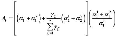 ,
,

 (59)
(59)
Proof. See Appendix B. ■
Using (59), the inter-temporal indirect utility function in Period 1 can be obtained as:
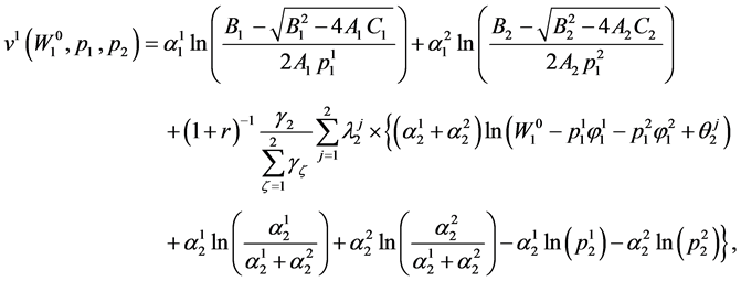
where  is as given in Proposition 7.1.
7.2. Wealth Compensated Demand
Following the analysis in Section 5 we obtain the wealth compensated demands in Period 2 as

for  and
and .
.
The expenditure function in Period 2 becomes:
 (60)
(60)
Now we proceed to Period 1. Following the analysis from Equation (37) to Equation (42) the wealth compensated demand function in Period 1 can be obtained as:
Proposition 7.2. The wealth compensated demand functions in Period 1 are:
 (61)
(61)
for  and
and .
.
Proof. See Appendix C. ■
Invoking the fact that

one can also have:

for  and
and . (62)
Proof. See Appendix C. ■
The wealth expenditure function in Period 1 can be expressed as:
 (63)
(63)
where  and
and  are given in (61).
7.3. Random Horizon Slutsky Equation
From (48) we obtain the stochastic dynamic Slutsky equations:
 (64)
(64)
To verify the duality results and Slutsky equations numerically we consider the illustration in this Section with the following parameter values: 


 ,
, 


 ,
,  and
and .
.
In Table 1, the results showing that the ordinary demand  equals the wealth-compensated demand
 , for
, for , are given in the first two rows. The indirect utility and wealth expenditure are given in the third row.
In Table 2, the results for the eight stochastic dynamic Slutsky equations
 for
for , are given as random horizon stochastic dynamic Slutsky Equations (1) to (8). The numerical values of partial derivatives are derived and the Slutsky results are shown in the last row of each equation block.
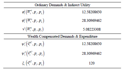
Table 1. Numerical depiction of wealth-dependent ordinary demands, wealth compensated demands, indirect utility and wealth expenditure.
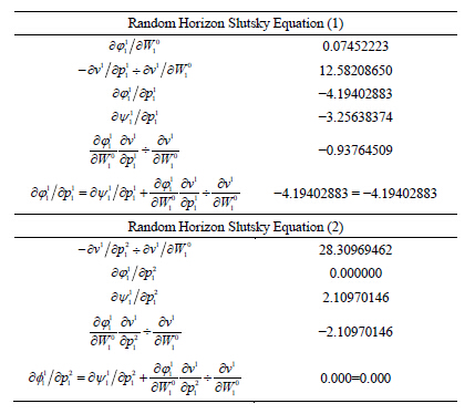
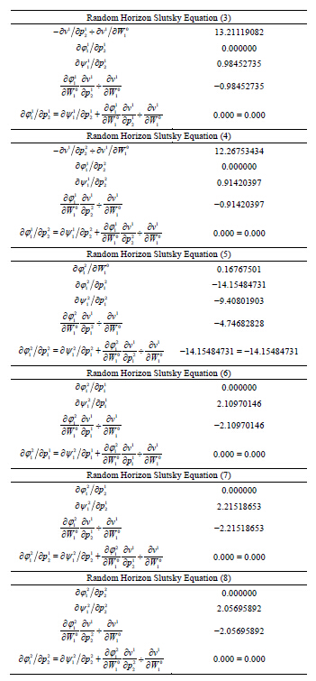
Table 2. Numerical depiction of the partial derivatives and random horizon stochastic dynamic slutsky equations.
8. Concluding Remarks
This paper extends the conventional consumer analysis to a random horizon stochastic dynamic framework in which the consumer has a planning horizon of  periods and there is uncertainty in future incomes and the consumer’s life span. The extension incorporates realistic and essential characteristics of the consumer into conventional consumer theory. The paper derives the Roy’s identity and Slutsky equation for this framework. It is the first time that the Roy’s identity is derived in an inter-temporal setting. With the Roy’s identity the random horizon stochastic dynamic Slutsky is presented in a more comprehensive form than the stochastic dynamic Slutsky equations of Yeung [8]. The analysis advances the microeconomic study on optimal consumption decision to a random horizon stochastic dynamic framework. Further research, development and propagations which explore further economic implications of the results in this paper are in order.
REFERENCES
- E. E. Slutsky, “Sulla Teoria Del Bilancio Del Consumatore,” Giornale Degli Economisti, Vol. 51, No. 1, 1915, pp. 1-26.
- R. G. D. Allen, “Professor Slutsky’s Theory of Consumers’ Choice,” Review of Economic Studies, Vol. 3, No. 2, 1936, pp. 120- 129.
- R. G. D. Allen, “The Work of Eugen Slutsky,” Econometrica, Vol. 18, No. 3, 1950, pp. 209-216.
- J. R. Hicks and R. G. D. Allen, “A Reconsideration of the Theory of Value. Parts 1-2,” Economica, New Series, Vol. 1, No. 1 & 2, 1934, pp. 52-76 & 196-219.
- H. Schultz, “Interrelations of Demand, Price, and Income,” Joumal of Political Economy, Vol. 43, No. 4, 1935, pp. 433-481.
- P. C. Dooley, “Slutsky’s Equation Is Pareto’s Solution. History of Political Economy,” Vol. 15, No. 4, 1983, pp. 513-517.
- T. W. Epps, “Wealth Effects and Slutsky Equations for Assets,” Econometrica, Vol. 43, No. 2, 1975, pp. 301-303.
- D. W. K Yeung, “Optimal Consumption under an Uncertain Inter-Temporal Budget: Stochastic Dynamic Slutsky Equations,” Vietsnik St Petersburg University: Mathematics, Vol. 10, No. 3, 2013, pp. 121-141.
- R. Roy, “La Distribution Du Revenu Entre Les Divers Biens,” Econometrica, Vol. 15, No. 3, 1947, pp. 205-225.
- M. L. Puterman, “Markov Decision Processes: Discrete Stochastic Dynamic Programming” John Wiley & Sons, New York, 1994. http://dx.doi.org/10.1002/9780470316887
- D. P. Bertsekas and S. E. Shreve, “Stochastic Optimal Control: The Discrete-Time Case,” Athena Scientific, 1996.
- D. W. K Yeung and L. A. Petrosyan, “Subgame Consistent Cooperative Solution of Dynamic Games with Random Horizon,” Journal of Optimization Theory and Applications, Vol. 150, No. 1, 2011, pp. 78-97.
- D. W. K Yeung and L. A. Petrosyan, “Subgame Consistent Solution for Cooperative Stochastic Differential Games with Random Horizon,” International Game Theory Review, Vol. 14, No. 2, 2012, pp. 1250012.01-1250012.22.
- R. Bellman “Dynamic Programming,” Princeton University Press, Princeton, 1957.
- M. T. Cheung and D. W. K. Yeung, “Microeconomic Analytics,” Prentice Hall, New York, 1995.
Appendices
Appendix A. Proof of Theorem 4.1
Invoking (22) we obtain the identity
 (65)
(65)
Differentiating (65) with respect to  yields:
 (66)
(66)
Using (32) we have
 (67)
(67)
Substituting (67) into (66) yields
 (68)
(68)
Invoking (29) we obtain:
 (69)
(69)
Using (69) the terms inside the square brackets in (68) can be written as
 (70)
(70)
Invoking the first order conditions in (23) the term inside the square brackets in (70) vanishes and therefore (68) becomes:
 (71)
(71)
Using (69), one has
 (72)
(72)
Substituting (72) into (71) yields
 (73)
(73)
Invoking (69) one obtains
 (74)
(74)
Dividing (73) by (74) yields another form of the random horizon Roy’s identity as:
 (75)
(75)
for  and
and .
.
Hence Theorem 4.1 follows. Q.E.D.
Appendix B: Proof of Proposition 7.1
The problem facing the consumer in period 1 can be expressed as:
 (76)
(76)
where 
Using the First order condition for a maximizing solution for (76) yields
 (77)
(77)
Upon rearranging terms (77) can be expressed as:
 (78)
(78)
Equation (78) can be reduced into a quadratic equation in  with roots
 , (79)
where ,
,
 and
and .
.
One can show that both roots are real and positive, and the smaller root yields a utility maximizing solution.
 . (80)
Following similar analysis,  can be obtained as in Proposition 7.1. Q.E.D.
Appendix C: Proof of Proposition 7.2
The consumer’s dual problem in period 1 can be formulated as minimizing
 (81)
(81)
subject to the constraint
 (82)
(82)
Setting up the corresponding Lagrange function of the problem and performing the relevant minimization yield the first order conditions

 (83)
(83)
where  is given in (57).
Invoking  and (60) one can readily obtain:
 (84)
(84)
Using (84), one can reduce the first two equations in (83) to:
 (85)
(85)
for .
.
Using (85), one obtains  and upon substituting into the last equation of (83) yields

which could be expressed alternatively as:
 (86)
(86)
Solving  from (86) yields the wealth compensated demand for good 1 as:
 (87)
(87)
Following the above analysis, the wealth compensated demand for good 2 can be obtained as that given in Proposition 7.2. Q.E.D.