Applied Mathematics
Vol.4 No.9A(2013), Article ID:36703,11 pages DOI:10.4236/am.2013.49A006
Hybrid Predictive Control Based on High-Order Differential State Observers and Lyapunov Functions for Switched Nonlinear Systems
1School of Electrical Information and Automation, Qufu Normal University, Qufu, China
2F’SATIE and Department of Electrical Engineering, Tshwane University of Technology, Pretoria, South Africa
Email: guoyuanqi@gmail.com, vanwykb@gmail.com
Copyright © 2013 Baili Su et al. This is an open access article distributed under the Creative Commons Attribution License, which permits unrestricted use, distribution, and reproduction in any medium, provided the original work is properly cited.
Received April 26, 2013; revised May 26, 2013; accepted June 4, 2013
Keywords: Switched System; Lyapunov Function; High Order Differentiator; Control Constraint; Output Feedback; Model Predictive Control; Stable Region
ABSTRACT
In this paper, a hybrid predictive controller is proposed for a class of uncertain switched nonlinear systems based on high-order differential state observers and Lyapunov functions. The main idea is to design an output feedback bounded controller and a predictive controller for each subsystem using high-order differential state observers and Lyapunov functions, to derive a suitable switched law to stabilize the closed-loop subsystem, and to provide an explicitly characterized set of initial conditions. For the whole switched system, based on the high-order differentiator, a suitable switched law is designed to ensure the whole closed-loop’s stability. The simulation results for a chemical process show the validity of the controller proposed in this paper.
1. Introduction
Switched system is a typical hybrid dynamic system made up of some subsystems and a switched law. In recent years, the stabilization of constrained switched systems became an attractive research subject [1].
Model predictive control (MPC) is a receding horizon control (RHC) method to handle constraints within an optimal control setting [2]. There have been many results to show the performance of constrained MPC [3]. In MPC design, the initial feasibility of the optimization problem is always assumed. Due to uncertainties and constraints of the practical process, this assumption may not be satisfied. Furthermore, the set of initial conditions, starting from where a given MPC formulation is guaranteed to be feasible, has not been explicitly characterized.
In recent years, controller design methods based on Lyapunov functions have been developed, which can give an explicitly characterized set of initial conditions from which the closed-loop system is stable [4]. By embedding the Lyapunov-based design methods into the MPC design, we can obtain the set of initial conditions from where the closed-loop system is stable. In refs. [5,6], two Lyapunov-based predictive controllers were derived for constrained nonlinear systems. In refs. [7,8], two Lyapunov-based predictive controllers were proposed for constrained switched systems and constrained switched systems with uncertainties, respectively. In these papers, the states of the system are observable.
However, in real processes the system’s states are often not measurable, and hence, state-feedback controllers and switched laws cannot be realized. One of the methods to overcome this difficulty is to construct a state observer to estimate the states for constructing the controller and switched law. In ref. [9], an output feedback bounded controller was given for a class of nonlinear systems which was not switched system. In ref. [10], for a kind of nonlinear switched systems without uncertainties and disturbance, a bounded nonlinear controller was given. But it was not guaranteed to be optimal with respect to an arbitrary performance criterion which incurporates requested performance in the design. In ref. [11], a hybrid output feedback predictive controller was proposed for a class of switched nonlinear systems without uncertainties. In papers [9-11], the processes’ states were estimated using a high-gain observer, but many adjustable parameters of the observer need to be chosen experientially. Sometimes the wrong selection of parameters can cause stability problems and an undesired transient performance of the observer. In refs. [12-14], a high-order differential state observer was designed to estimate the states of a nonlinear system. Theoretically the parameters are chosen according to the performance and stability of the observer and theoretically few parameters with explicit meanings have to be selected based on the performance and stability of the observer.
In this paper, an output feedback hybrid predictive controller is proposed for a class of uncertain switched nonlinear systems based on high-order differential state observers and Lyapunov functions. The main idea is to design a hybrid predictive controller based on Lyapunov functions and high-order differential state observers, which switches between a bounded feedback controller and a predictive controller for each subsystem, and to provide an explicitly characterized set of initial conditions to stabilize the closed-loop subsystem. Here, we use high-order differentiators as state observers. This high-order differential state observer has simple structure with few parameters. A suitable switched law based on the high-order differentiator is designed to guarantee the whole closed-loop system’s stability. Finally, the simulation results for a chemical process show the validity of the procedure proposed in this paper.
2. Problem Description
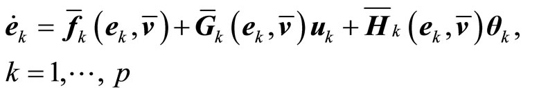
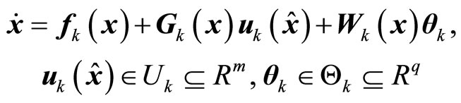
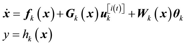
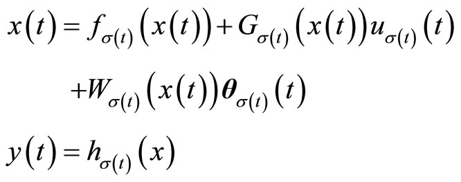
Consider the constrained switched nonlinear system
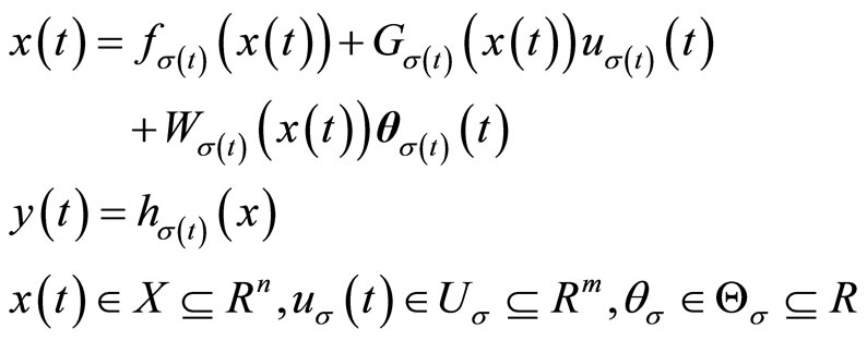 (1)
(1)
where  denotes the vector of continuous-time state variables,
  is the set containing the states;
 denotes the vector of manipulated inputs taking values in a nonempty compact subset
 , where
  is the Euclidian norm, and
  is the magnitude of the constraints.
  denotes the measured output;
  is a sufficiently smooth function;
 denotes the bounded uncertain parameter vector taking values in a nonempty compact subset
 ;
;
 is the switching signal assuming to be a piece-wise continuous (from the right) function of timei.e.,
  for all
 , implying that only a finite number of switches is allowed on any finite interval of time, and
  is the number of modes of the switched system. Throughout this paper, we use the notations
  and
and  to denote the time at which, for the rth time, the kth subsystem is switched in and out, respectively, i.e.,
 . With this notationit is understandable that the continuous state evolves according to
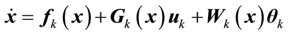 ,
,
 , for
, for .
. and
and
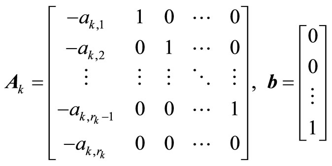
 denote the set of switching times at which the kth subsystem is switched in and out, respectively. It is assumed that all entries of the vector functions
 , the n × m matrices
  and the n × q matrices
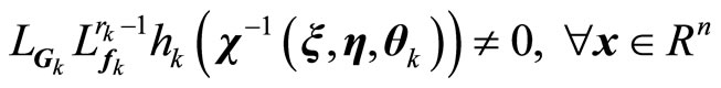
  are sufficiently smooth and that
 for all
 . In this paper, the notation
 denotes the standard Lie derivative of a scalar function
  with respect to the vector function
 :
: , and
, and
 .
.
The objective of this paper is to design a nonlinear output feedback predictive controller based on Lyapunov functions and a high order differential state observer for the case where state measurements are not available for each mode of the uncertain switched nonlinear system given by Equation (1). Then, for the whole switched system, based on state estimations, a suitable switched law is designed to ensure the whole closed-loop system’s stability.
3. Preliminaries
3.1. High-Order Differential State Observers
In order to construct an output feedback controller to stabilize the controlled system (1), we use high-order differential state observers [12-14] to estimate the unmeasurable states of the system (1).
Firstly, we give some assumptions.
Assumption 1: Consider system (1), for every , there exist an integer
  and a set of invertible coordinates
 (2)
(2)
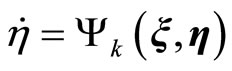
where 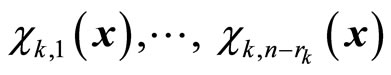 are nonlinear scalar functions of x, such that the system (1) takes the form
 (3.1)
(3.1)
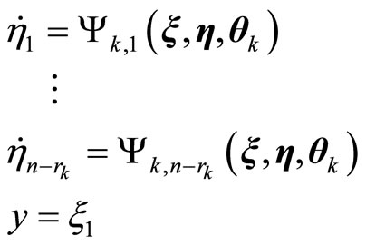 (3.2)
(3.2)
where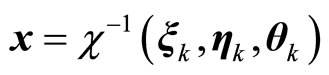 ,
,
 , and
, and
 are nonlinear functions describing the corresponding evolution of the kth inverse dynamics mode, and
 if and only if
 .
.
Assumption 2: The dynamical  subsystem in (3)
 (4)
(4)
is input-to-state stable (ISS) [9], where
 and
and .
.
The following assumptions are given to reduce the influence of uncertainties.
Assumption 3: There exists a known constant  such that
 .
.
Assumption 4: For each , a control Lyapunov function
  exists.
Before designing the output feedback controller, we have to revise Assumption 1.
Assumption 5: There exists an invertible coordinate transformation , such that system (1) takes the form similar to (3) in which the
  tem take the following form
 (5)
(5)
This formula is different from formula (4) since it does not depend on the uncertain parameter . We also assume this subsystem is ISS stable.
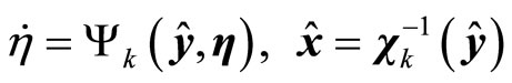
In order to construct a controller to stabilize the controlled system (1), we use high-order differential state observers [12-14] to estimate the un-measurable states of system (1). The high-order differential state observer for each mode can be described as
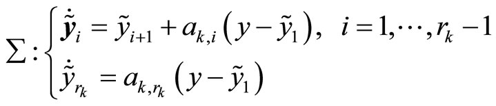 (6)
(6)
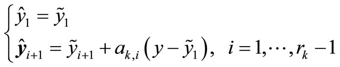 (7)
(7)
where 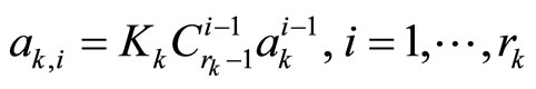
 (8)
(8)
Here  denotes the combination expression and only one parameter
  is adjustable, all other parameters
  can be calculated using
  and
and . Clearly,
  is the only external input of system
 , so we can obtain
  based on the measured signal
  via (6), and further calculate the estimated derivatives
  via (7). Note that the HOD is independent of the model of the original system (1).
Proposition 1. The HOD does not rely on the model of the estimated system, parameters are chosen using (8), and has following characteristics:
1) The HOD is an asymptotically stable system.
2)
 (9)
(9)
3.2. State Feedback Bounded Controller Based on Lyapunov Functions
We recall the design of a state feedback bounded controller to obtain the set of initial conditions from which the system is stable [9].
Define the tracking error variables
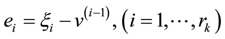 and the tracking error vector
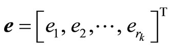 ,
, 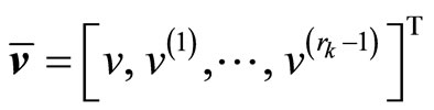 is the reference input vector, where
  is a reference input and
  is its ith time derivative. Then the
  in system (3) can be re-written as
 (10)
(10)
where 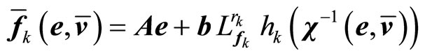 is a
is a 
vector function, 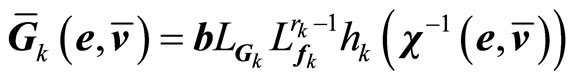 is a
is a
 matrix function,
 is a
is a  matrix function, and
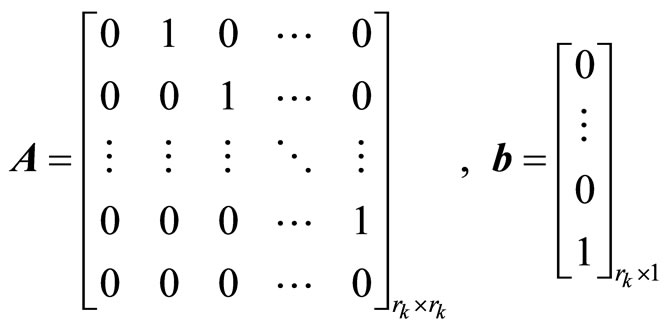 . (11)
The Lyapunov function is chosen as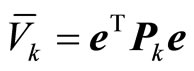 , where the positive-definite matrix
  is chosen to satisfy the following Ricatti inequality
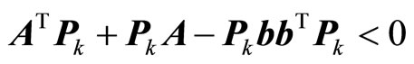 (12)
(12)
Definition 1.  is a class
  function if it is a strictly increasing function satisfying
 .
.
Definition 2. Function  is a class
  function, if
 ,
,  is non-increasing, and
 ;
; ,
,  is non-increasing, and
 .
.
Choose a class  function
  that satisfies
 and define the set
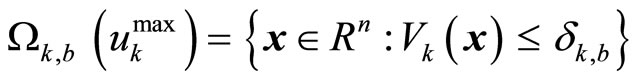 , where
is satisfying , where
 is a class
  function.
The continuous bounded control law is constructed as follows [9]
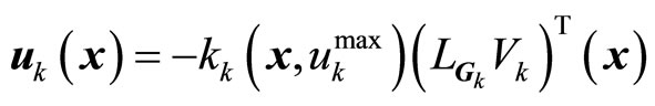 (13)
(13)
with
 (14)
(14)
where
 ,
,
 ,
,
 ,
,
 and
and
 are row vectors, where
 is the
  column of
  and
and  is the
  column of
 ;
; ,
,  ,
,  are adjustable parameters.
Remark 1. For convenience, this bounded controller (13)-(14) is redefined as .
.
Remark 2. Here, the Lyapunov functions used in verifying the switching conditions at any given time,  , are based on
 . Note that the Lyapunov functions
  are in general different from
  used in bounded controllers. For the systems with relative degree
 , the choice of
  is sufficient.
Based on this bounded controller (13)-(14), an estimation of the stability region is computed as
 (15)
(15)
where  is the largest number for which
 , and
, and
 . (16)
The robustness property of the bounded controller in (13)-(14) is formalized by the following proposition:
Proposition 2. Consider the system (1) for a fixed value . Under the Assumptions 1-4, compute the bounded control law of (13)-(14) using the Lyapunov functions
  and
and , and then give the stability region estimate
 . Let
. Let ,
,
 , where
 ,
,
 . Then, given any positive real number
 , there exists positive real numbers
 , such that if
  and
and , then
 , and
, and . Furthermore, if
 , then
 ,
,
 ; if
; if , then
 ,
,  and the output of the closedloop system satisfies:
  (The proof is similar to the proof of Theorem 1 in ref. [9]).
3.3. Output Feedback Bounded Controller Based on State Estimations and Lyapunov Functions
In this section, we consider the case when some states of system (1) are not measurable. The bounded controller based on state estimations and Lyapunov functions should be designed and the stable region of initial conditions should be described.
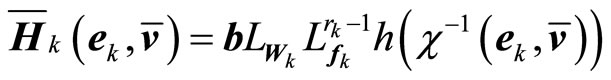
Based on the high-order differential state observer (6)- (8), the following presents the output feedback controller used for each mode and characterizes its stability properties:
Proposition 3. Considering the nonlinear system (1), for a fixed mode , design the output feedback controller with a high-order differential state observer (6)-(8)
 (17)
(17)
where ,
,  ,
,
 are vectors with dimension
 .
.
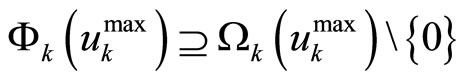
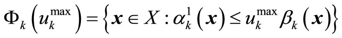
Given , where
  is a class
  function and
  is the maximum value of
 for
for and
and , such that if
 , then, given
 there exists
 , such that if
 ,
,
 and
and , the origin of the closedloop system is asymptotically (and locally exponentially) stable, i.e., there exists
 , such that
 . Furthermore, given
  and some real number
 , there exists a real number
 such that
 , for
, for . Andthe output of the closed-loop system satisfies
 (This proposition is a special case of Theorem 2 in ref. [9]).
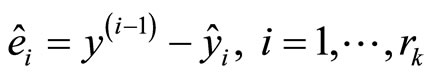
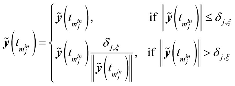
Remark 3. Here, a high order differential state observer is used to provide the estimates of the derivatives of the output y up to order , denoted as
 , and thus estimates of the variables
 (note from Assumption 1 that
 ). This high-order differentiator has only one adjustable parameter. To eliminate the peaking phenomenon associated with the high order differential states observer, a standard saturation function
  is introduced to eliminate wrong estimates of the output derivatives, or alternatively the following formulation can be used [12-14]
 (18)
(18)
where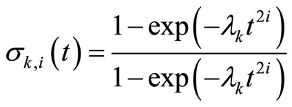 .
.
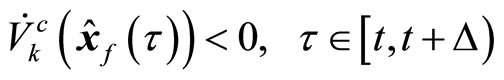
Remark 4. The ith closed-loop subsystem can be cast as a two time-scale system given by
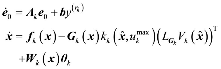 (19)
(19)
where e0 is a vector of the auxiliary error variables
 , and
, and
 (20)
(20)
Proposition 4 establishes the existence of a set,  , such that once the state estimation error is smaller than a certain value (note that the decay rate can be controlled by adjusting
 ), the presence of the state is within the output feedback stability region,
 .
.
Proposition 4. Given any positive real number , there exist positive real numbers
 ,
,  , and a set
 such that if
 , where
 , then
 .
.
4. Integrated Predictive Controller Design Based on State Estimation and Lyapunov Functions
4.1. Predictive Controller Design Based on State Estimation and Lyapunov Functions for Every Subsystem
A MPC based on the high-order differential state observer and Lyapunov functions will be designed for system (1) with a fixed 
 in this section. The control action at time
  and state estimation
  are conventionally obtained by on-line solving a finite horizon optimal control problem described as
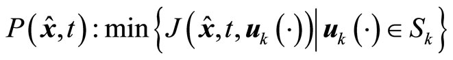 (21)
(21)
 (22)
(22)
 (23)
(23)
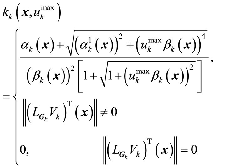
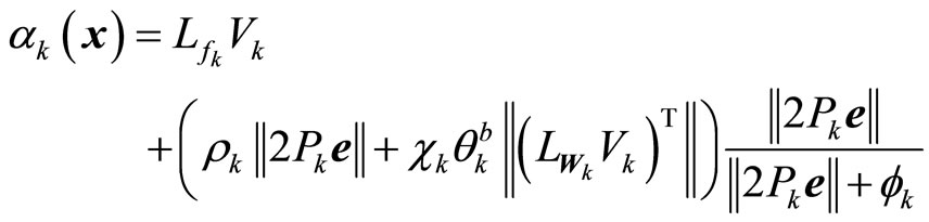
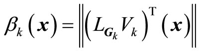
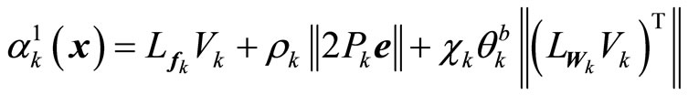
where

 (24)
(24)
 (25)
(25)
 (26)
(26)
 , (27)
 (28)
(28)
 (29)
(29)
 . (30)
Here ,
,  are defined in Proposition 1,
  are defined in Proposition 2 and
 .
.
 is a family of piecewise continuous functions (from the right), with period
 , mapping
  into the set of admissible controls
 .
.  is the horizon length and
  is the Lyapunov function used to design bounded controller.
  is the Lyapunov function of the system. A control
  in
in  is characterized by the sequence
 ,
,  and satisfies
  for all
 . The performance index is given by
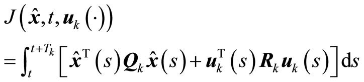 (31)
(31)
where  and
and  are positive semi-definite and strictly positive definite symmetric matrices, respectively. The optimal control
  is then applied to the plant over the interval
  and the procedure is repeated indefinitely. This defines an implicit model predictive control law
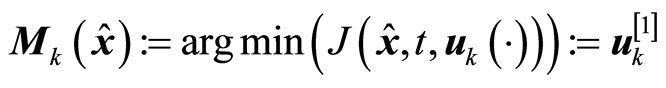 (32)
(32)
Owing to the existence of parameter uncertainties and constraints, the initial feasibility of the MPC in (32) is not guaranteed. If it is infeasible, the control action is switched to the bounded controller (17). To describe the whole control action, we cast the kth subsystem (1) as a switched system of the form
 (33)
(33)
where 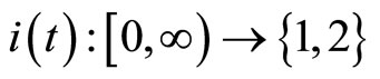 is the switching signal which is assumed to be a piecewise continuous (from the right) function of time. When
 , the control input takes
 , i.e., the MPC is used; and when
 , it takes
 , i.e., the bounded control is used.
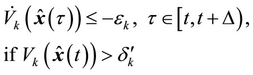
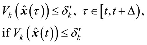
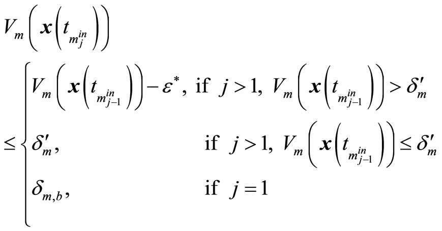
Proposition 5. Consider the switched nonlinear system in (33). For a fixed , the control action is switched between the model predictive controller (21)- (31) and the bounded controller (17). Let
 . At the earliest time
 when the closed-loop system’s states under MPC satisfy
 , set
, set ; at the earliest time
 when the states under MPC satisfy
 , set
, set ; at the earliest time
  when the states under MPC satisfy
 , set
, set ; at the earliest time
  when MPC is infeasible, set
 . Define
 , where
  is a designed time arbitrary. Then, the switching rule
 (34)
(34)
guarantees the stability of the closed-loop subsystem (see the proof in Appendix A).
Remark 5. The mixed predictive controller above is designed and implemented using the following steps:
1) For the subsystem (1) with a fixed
 , design the bounded controller (17), and compute the stable region
 ;
;
2) Design the MPC controller given by (21)-(31);
3) Given initial conditions  and
and
 , implement the MPC controller given by (21)-(31) if it is feasible;
4) When the MPC is infeasible , or the state estimation
  of the closed-loop subsystem reaches the boundary of
 , i.e., when
 , or
, or
 satisfies
 , or
, or
 , the controller switches to the bounded controller given by (17) until the MPC is feasible again or until the designed switched time
 ;
;
5) When another subsystem is switched in, go to step 1).
Remark 6. The purpose of switching to the bounded robust controller after the time  is to ensure convergence and avoid possible cases where the closed-loop states, under MPC, could wander inside
  without actual convergence.
4.2. Integrated Design of the Controller and the Switched Law for the Whole Switched System
Consider the constrained switched nonlinear system (1) with parameter uncertainties and definite switched time sequences  and
and
 . Theorem 1 gives the switched law that ensures the stability of whole closed-loop system.
Theorem 1. Consider the switched nonlinear system (1) for which there exist control Lyapunov functions ,
, . Given any initial conditions
  and
and , where
  was defined in Proposition 1, and chosen positive real numbers
 , compute the stable region estimation
 . Choose
  to compute
 . Choose
  such that
 . Let
. Let
 be the design time and t satisfy
 . Assume
  for some
 . The mixed controller switched between the bounded controller (17) and the MPC (21)-(31) is designed with the switched law (34), such that if
 (35)
(35)
 (36)
(36)
 (37)
(37)
then the whole closed-loop system is stable (See the proof in Appendix B).
Remark 7. The controller presented in Theorem 1 can be implemented using the following steps:
1) Given the system model (1) with constraints on the inputs, and a control Lyapunov function  to design the bounded controller (17) with suitable parameters and compute the stability regions (15) and (16). Here the stability regions are only signs, for the states cannot be measured, and in the controller design only the stable region estimation
  is used. And choose Lyapunov function
  for the system (19);
2) Determine suitable parameters to design the MPC in (21)-(31). Give the size of the ball to which the state is required to converge,  , and compute
 such that for every subsystem it has
 . Compute
 , and choose
 , for a real positive number
such that ;
;
3) For time  (the rth time of switching into the kth subsystem), consider whether the state estimation belongs to the stable region
 ;
;
4) Pick  in the switched sequence;
5) At the time of switching in the mth subsystem, consider the constraints in Theorem 1, and choose  and
and  satisfying (36) and (37), respectively;
6) When the mth subsystem is switched in, the constraint  is required to be satisfied. If
 ,
, ; if the state is in the neighborhood of origin, then
and . If constraint (37) is used to ensure
 , then
  and the closed-loop system is stable according to Proposition 4.
Remark 8. [10]. The time interval between two consecutive switches should be long enough to ensure that the estimation error decreased to a sufficiently small value such that the closed-loop system is stable. Furthermore, the decision to switch is not based on  , but rather based on
  (under state feedback it was based on
 ). If
). If  at some early time, a switch is not executed before
 .
.
5. Simulation
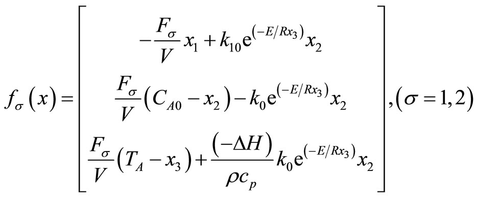
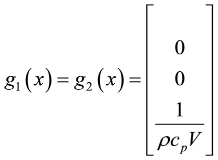
Consider a continuously stirred tank reactor where three parallel, irreversible, first-order exothermic reactions of the form 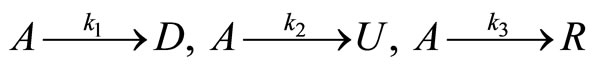 take place, where A is the reactant species, and
  is the desired product species, U, R denote the by-product species. Under standard modeling assumptions, the mathematical model for the process takes the form [8]
 (38)
(38)
where  and
and  denote the concentration of species A and D, respectively. T denotes the temperature of reactor.
  is the rate of heat input to the reactor. V the volume of the reactor.
  denote the pre-exponential constants, the activation energies. And the enthalpies of the three reactions, respectively,
  and
and  are the heat capacity and density of the fluid in the reactor.
  is the switched variable. The values of these parameters can be found in Table 1.
The control objectives are to: (1) stabilize the reactor temperature at the open-loop unstable steady state Ts = 388.58 K of mode 1, and (2) maintain the temperature at this steady-state when the reactor switches to mode 2. The control objective is to be accomplished in the presence of: (1) exogenous time-varying disturbances in the feed stream temperature, (2) parametric uncertainty in
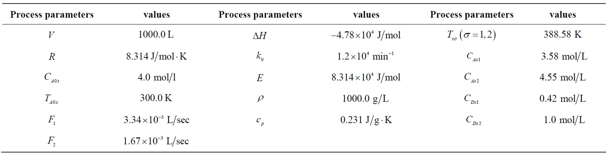
Table 1. Process parameters and steady-state values.
the enthalpy of the three reactions, and (3) hard constraints on the manipulated inputs.
Note that, with this requirement, both closed-loop modes share the same steady-state temperature but have different steady state reactant concentrations. The control objective is to be accomplished by manipulating Q provided by the jacket, subject to the input constraint .
.
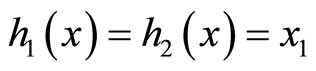
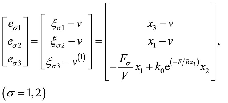
Defining 
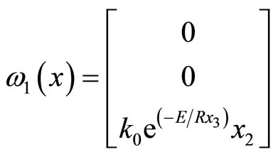
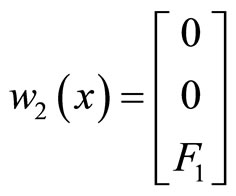
 , y = x1, the process model of Equation (34) can be cast in the form of Equation (1)
where
 ,
,
 ,
,  ,
,
 ,
, .
.
The boundary of parameters is ,
, . For this system, perform the following coordinate transformation
 (39)
(39)
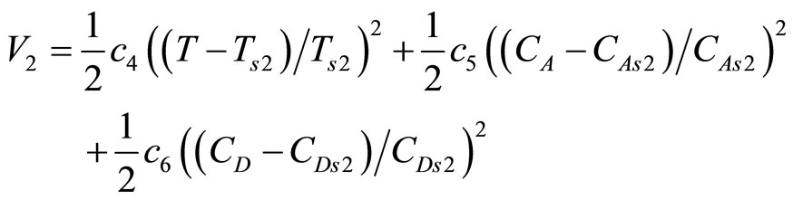
Two quadratic, positive-definite functions of the form,
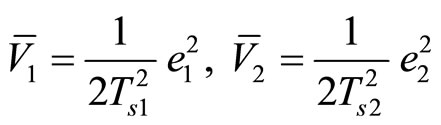 , are then used to synthesize two bounded nonlinear controllers (one for each mode) of the form
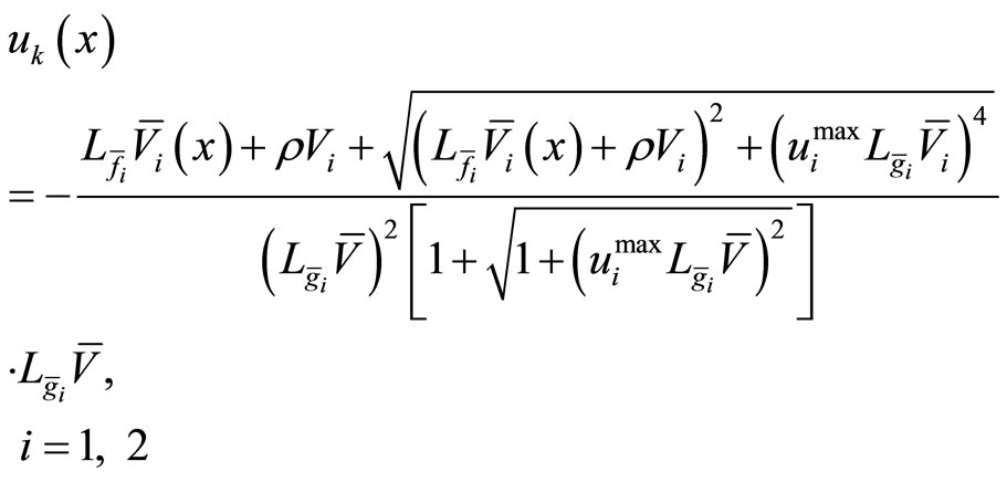
(40)
Note that these positive-define function is given for system (39). To estimate the stability regions, the Lyapunov functions
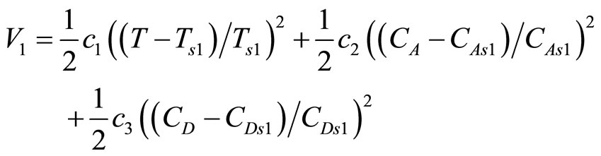
where ,
,  ,
, ; and
; and
where , are used.
Given initial state , and switched time
 , the parameters of the high-order differential state observer take as
 . Using the hybrid MPC method proposed in this paper, we obtained the following simulation results:
In the simulation, starting from mode 1, the predictive controller was first implemented before switching to the bounded controller at . At the designed switched time
  the system turned to mode 2. In mode 2, the predictive controller was first implemented before switching to the bounded controller at
  and at
  it was again switched to predictive controller.
Figures 1 to 4 demonstrate the validity of the controller proposed in this paper.
6. Conclusion
In this paper, a hybrid predictive control method is pro-
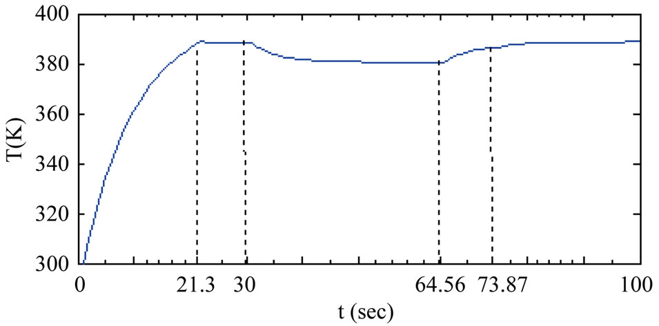
Figure 1. Closed-loop state (the reactor temperature T) profile.
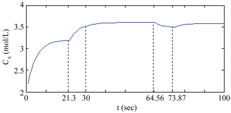
Figure 2. Closed-loop state (the reactor concentration CA) profile.
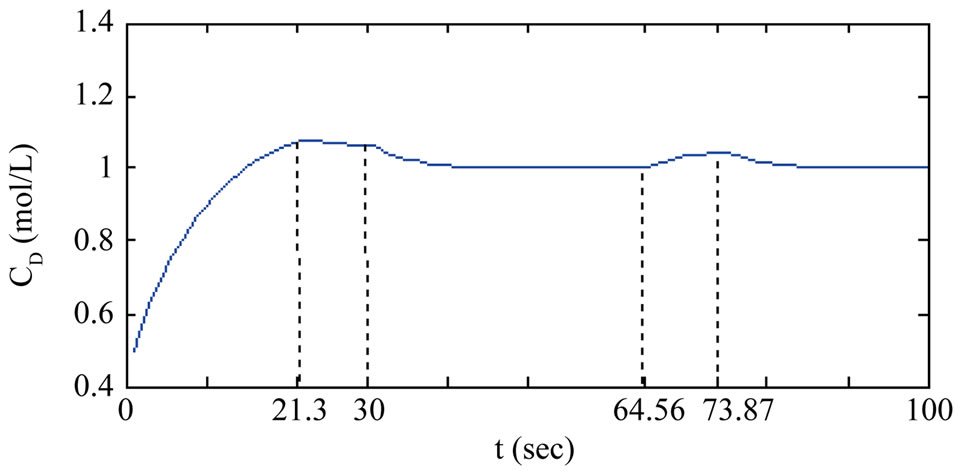
Figure 3. Closed-loop state (the reactor concentration CD) profile.
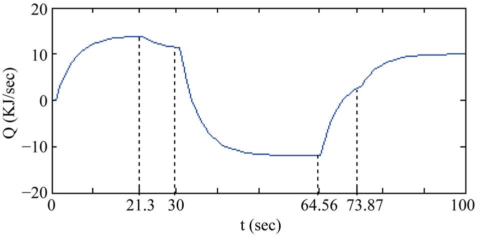
Figure 4. The input Q profile.
posed for a class of uncertain switched nonlinear systems with input constraints and unavailable state measurements. The main objectives were to design a hybrid controller which switches between a bounded controller and a predictive controller based on Lyapunov functions and a high-order differential state observer with a suitable switched law to stabilize the closed-loop subsystem, and to provide an explicitly characterized set of initial conditions. For the whole switched system, a suitable switched law based on the state estimation was derived to ensure the whole closed-loop system’s stability. The simulation results for a continuously stirred tank reactor showed the validity of the controller proposed in this paper.
7. Acknowledgements
This work was supported by the National Natural Science Foundation of Peoples Republic of China under Grants 61374004, 61004013, 61104007 and 60804033, the National Specialized Research Fund for the Doctoral Program of Higher Education under Grant 20113705120003, Higher Educational Science and Technology Program Foundation of Shandong Province under Grant J10LG28, J11LG08 and the Doctoral Starting Research Fund from the Qufu Normal University.
REFERENCES
- J. Hespanha and A. S. Morse, “Switching between Stabilizing Controllers,” Automatica, Vol. 38, No. 11, 2002, pp. 1905-1917. doi:10.1016/S0005-1098(02)00139-5
- S. L. D. Kothare and M. Morari, “Contractive Model Predictive Control for Constrained Nonlinear Systems,” IEEE Transactions on Automatic Control, Vol. 45, No. 6, 2000, pp. 1053-1071. doi:10.1109/9.863592
- D. Q. Mayne, J. B. Rawlings and P. O. M. Rao, “Constrained Model Predictive Control: Stability and Optimality,” Automatica, Vol. 36, No. 6, 2000, pp. 789-814. doi:10.1016/S0005-1098(99)00214-9
- M. S. Branicky, “Multiple Lyapunov Functions and Other Analysis Tools for Switched and Hybrid Systems,” IEEE Transactions on Automatic Control, Vol. 43, No. 4, 1998, pp. 475-482. doi:10.1109/9.664150
- P. Mhaskar, N. H. El-Farra and P. D. Christofides, “Robust Hybrid Predictive Control of Nonlinear Systems,” Automatica, Vol. 41, No. 2, 2005, pp. 209-217. doi:10.1016/j.automatica.2004.08.020
- P. Mhaskar, N. H. El-Farra and P. D. Christofides, “Stabilization of Nonlinear Systems with State and Control Constraints Using Lyapunov-Based Predictive Control,” Systems and Control Letters, Vol. 55, No. 8, 2006, pp. 650- 659. doi:10.1016/j.sysconle.2005.09.014
- P. Mhaskar, N. H. El-Farra and P. D. Christofides, “Predictive Control of Switched Nonlinear Systems with Scheduled Mode Transitions,” IEEE Transactions on Automatic Control, Vol. 50, No. 11, 2005, pp. 1670-1680. doi:10.1109/TAC.2005.858692
- S. Baili and L. Shaoyuan, “Constrained Predictive Control for Nonlinear Switched Systems with Uncertainty,” Acta Automatica Sinica, Vol. 34, No. 9, 2008, pp. 1141- 1147
- N. H. E1-Farra and P. D. Christofides, “Bounded Robust Control of Constrained Multivariable Nonlinear Processes,” Chemical Engineering Science, Vol. 58, No. 13, 2003, pp. 3025-3047. doi:10.1016/S0009-2509(03)00126-X
- N. H. E1-Farra, P. Mhaskar and P. D. Christofides, “Output Feedback Control of Switched Nonlinear Systems Using Multiple Lyapunov Functions,” Systems & Control Letters, Vol. 54, No. 12, 2005, pp. 1163-1182. doi:10.1016/j.sysconle.2005.04.005
- B. L. Su, S. Y. Li and Q. M. Zhu, “The Design of Predictive Control with Characterized Set of Initial Condition for Constrained Switched Nonlinear System,” Science in China Series E-Technological Sciences, Vol. 52, No. 2, 2009, pp. 456-466. doi:10.1007/s11431-008-0249-8
- G. Y. Qi, Z. Chen and Z. Yuan, “Adaptive High Order Differential Feedback Control for Affine Nonlinear System,” Chaos, Solitons & Fractals, Vol. 37, 2008, pp. 308-315. doi:10.1016/j.chaos.2006.09.027
- G. Y. Qi, Z. Chen and Z. Yuan, “Model Free Control of Affine Chaotic System,” Physics Letters A, Vol. 344, No. 2-4, 2005, pp 189-202. doi:10.1016/j.physleta.2005.06.073
- G. Y. Qi, M. A. van Wyk and B. J. van Wyk, “Model-Free Differential States Observer for Nonlinear Affine System,” The 7th IFAC Symposium on Nonlinear Control Systems, 21-24 August 2007, Pretoria, pp. 984-989
Appendix A
Proof of Proposition 4
The proof uses the result of Proposition 3, if the bounded controller (17) is switched to, the state estimation of the closed-loop system resides in , i.e., there exist
 , such that
 . Here, the high-order differential state observer is used to estimate states of the controlled system; it is able to converge to the state evolution of the controlled system. So we can have
 , then
 , using the result of Proposition 4, we have
  and
and .
.
Therefore, we need only show that under the MPC (21)-(31), the closed-loop system is stable until the bounded controller is switched to. In order to do this, we consider five possible values of  to show that
 . Owing to the constraints (28)-(29), if
 , we can have
 . Since
 , we can have
 , so the closed-loop subsystem is stable.
Now, we show  for all the possible values of
 .
.
Case 1. If  (
( is the earliest time when states under MPC satisfy
 ), then we can have
 . By continuity of the solution of system (1), we have
 , i.e.,
 .
.
Case 2. If  (
( is the earliest time when states satisfy
 ), as long as dk is small enoughwe can have
 , i.e.,
 .
.
Case 3. If , then from the definition of
 , we can have
 . We proceed by contradiction to prove
 . Assume
 , then
 . Owing to continuity of the solution and
 , also since the fact
 , there exists a time
 for which
 . Since
 is the earliest time for which
 , it must be true that
 , which leads to a contradiction with
 . Therefore we can have
 .
.
Case 4 and Case 5. If  or
or , we can prove
  similar to Case 3 only need to replace
  by
by , and
, and , respectively.
By Proposition 4, we have , and
, and . This completes the proof of Proposition 5.
Appendix B
Proof of Theorem 1. (Similar to the proof of Theorem in ref. [7])
Based on Propositions 3-5, we need only to prove that, with the switched law (35)-(37), the whole closed-loop system is still stable.
Let t satisfy  and
and . For the active mode k, constraint (35) ensures the initial conditions switched on mode k, using the result of Proposition 5, we can have the mode k is stable. So we need only to prove the stability at the switched time.
If , using the constraint (28), we can have
 . While the constraint (35) ensures that
  if this mode is switched out and then switched back in. So we can have
 . Owing to the feasibility of constraints (28)-(29), then the value of
  continuously decreases. If this mode is not switched in, there exists at lease some
  such that mode
  is active and Lyapunov function
  continues to decrease until
 . Similar to discussion before, the constraint (35) ensures that
  continues to be less than
 . Hence,
 . The switched condition (37) ensures the boundedness of
  at switched transition time, so
 . This completes the proof of Theorem 1.