Applied Mathematics
Vol. 3 No. 6 (2012) , Article ID: 20083 , 6 pages DOI:10.4236/am.2012.36081
An Analysis of Heat Explosion for Thermally Insulated and Conducting Systems
1Department of Mathematical Sciences, Clemson University, Clemson, USA
2Department of Mechanical Engineering, Clemson University, Clemson, USA
3Department of Materials Science and Engineering, Clemson University, Clemson, USA
Email: {iviktor, mjscrug, izeller, kfairch}@clemson.edu
Received March 1, 2012; revised May 10, 2012; accepted May 17, 2012
Keywords: Computational Analysis; Conducting System; Heat Explosion; Heating Parameters; Insulated System; Self-Heating; Thermal Failure
ABSTRACT
In the scope of material science, it is well understood that mechanical behavior of a material is temperature dependent. The converse is also true and for specific loading cases contributes to a unique thermal failure mechanism known as “heat explosion”. The goal for this paper is to improve the mathematical models for predicting heat explosion by using a specific case of the Fourier heat transfer system that focuses on thermoviscoelastic properties of materials. This is done by using a computational analysis to solve for an internal heat parameter that determines thermal failure at a critical value. This critical value is calculated under conditions either accounting for or negating the effect of heat dissipated by the material. This model is an improvement on existing models because it accounts for material specific properties and in doing so limits mathematical assumptions of the system. By limiting the assumptions in the conditions of the model, the model becomes more accurate and useful in regards to material design.
1. Introduction
Material failure is a well researched branch of material science, and although most failure mechanics are observed in terms of crack initiation and subsequent crack propagation, the exact situations determining material failure can become much more complicated. One such complication occurs when the mechanism of loading the material is not longer a static condition but becomes a repeated pattern of loading and unloading [1]. In the case of polymeric material and composites there are special cases where the viscous resistance of the material can generate an internal thermal energy proportionate to both the magnitude and frequency of loading [2]. These phenomena can be seen in past studies with respect to tension compression testing of glass reinforced plastic [3].
The two primary laws of heat conduction, Fourier’s law of heat conduction and Maxwell’s heat conduction law, dictate that heat will diffuse proportionally to temperature from high to low concentrations. Under ordinary conditions the thermal energy is dissipated at approximately the same rate at which it is generated creating a stationary thermal state, however, in cases where there exists an imbalance of energy for which the heat generated is significantly greater than the heat dissipated. This builds heat up inside the material leading to a phenomenon known as “Heat Explosion”.
Heat explosion is a catastrophic failure of the material analogous to what would be expected from the sudden heat flux of an exothermic chemical reaction. The focal point of heat explosion theory is the idea that although mechanical behavior of a material can lead directly to fatigue failure, failure can also occur less intuitively in the form of thermal failure [4].
Cyclic loading occurs in engineering applications ranging from aviation composite steel to automotive engine walls and artificial knee joints. The ultimate goal in material selection and design for any of these applications is to be able to model and predict the occurrence of thermal failure in the form of heat explosion. In order to do this in increasingly complex systems, it is common practice to simplify the conditions of the system by making assumptions on parameters for both the environment and the material. Although these assumptions make the model more manageable in terms of feasibility and complexity, they inherently detract from the significance and accuracy of the result. For this reason the goal of this paper is to develop a model that can predict heat explosion while limiting assumptions regarding the condition of the system and in doing so, increasing the accuracy and usefulness of the model.
The novel approach regarding the model proposed by this paper lies in its ability to predict thermal failure using material properties, and in doing so limiting the parameters that need to be assumed. This paper elaborates on the connection that can be established between mechanical properties and thermal properties of a material. These properties can be collectively referred to as properties of thermoviscoelastic parameters. Using standard material creep testing, material specific parameters can be established empirically and applied using the ideas of Fourier’s law of heat conduction. Because this model focuses heavily on mechanical properties of a material, it is possible to devise a model that reduces the amount of required assumptions of the system and in doing so the model becomes both more effective and more significant.
There are three main material parameters factored into this model. The material property for heat retained by the system under cyclic loading (γ), the material property for heat dissipated by the system (β) and the material property for influence of the heat on the material (δ). There also exists a delta critical (δ*) which represents a unique condition of δ at the instant prior to heat explosion [5]. T represents the temperature of the system while Tm is the temperature of the material. Eta (η) is defined as the ratio of T to Tm and is used in the integration equations [5]. Although these are defined parameters, it is very difficult to give a physical manifestation of their meaning. For the time being these are all represented as unitless material parameters that will be given concrete meaning in work to be done in the future [5].
2. Governing Equations and MATLAB Computations
2.1. Modeling Equations
The modeling equations for most heat transfer processes can be derived from Fourier’s Law of Heat Conduction. The equations for this specific study match the Fourier system developed by Viktorova [6].
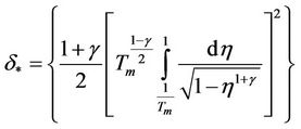 (1)
(1)
This equation is used to find the critical heat influence within a material that causes heat explosion, delta critical. In this case, heat removal is assumed to be zero. This represents a perfectly insulated scenario where no heat is dissipated. The right side of the equation is a Cauchy problem setting in terms of Tm. Tm must also satisfy the boundary conditions of the specimen in order to accurately model the physical sample. The Cauchy process is used to find delta critical as Tm is increased towards infinity [6]. The heat influence value rises quickly until the instant of heat explosion and then rapidly declines. For any specimen, heat explosion occurs at only one temperature and that temperature is only dependent on gamma. This is important because it validates comparison when beta is no longer zero. The next equation models that situation (see Equation (2)).
In most applications, self-heating materials have surrounding fluid flow or other cooling methods in place to prevent overheating and heat removal cannot be discarded. The equation above includes the removal of heat from the system by adding the beta term. Now, all three parameters have been committed to the system. The same Cauchy process is used here in order to find the delta critical values of the systems without perfect insulation.
2.2. MATLAB Conversion
The MATLAB program used for computation utilizes “quad”, “max” and “plot” functions as well as “for” loops to process and record the necessary data. MATLAB is convenient for this process because it can quickly compute the integrals found in (1) and (2). The following code represents (1).
fun20= @(n)
(1./(sqrt(1n.^(1+gamma))));
z1=quad(fun20,1/k,1);
Eq20(1,i)=((1+gamma)/2)*((k^((1-gamma)/2))*z1)^2;
Similarly, (2) becomes fun21= @(T) (1./(sqrt(((k.^(1+gamma))-(T.^(1+gamma)))+(((beta*(1+gamma))./2).*(T-k).*(T+k-2)))));
z2=quad(fun21,1,k);
Eq21(1,i)=(z2^2)*((1+gamma)/2);
MATLAB is also useful because it accepts anonymous functions. This allows the program to process the entire range of gammas and betas through the same function consecutively which reduces computation time and makes the program more efficient.
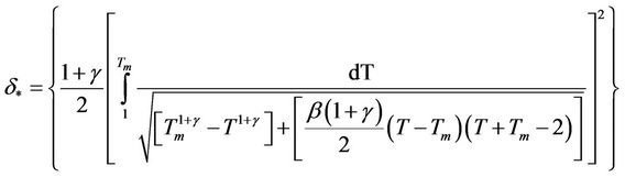 (2)
(2)
2.3. Comprehensive MATLAB Code
In this case, numerical computation is used to make solving the governing equations simpler. The MATLAB program uses input ranges of beta and gamma and solves delta critical for each unique pair. The program records these values in matrices that can be used for plotting. The method chosen to compare the data is one of ratios. A delta critical ratio is found, for each gamma and beta pair, which compares delta critical of a system with heat removal to one without. The ratio compares (1) and (2) for each pair in the input range.
3. Results and Discussion
3.1. Delta Critical
Figure 1 displays delta values based on the heat in the system Tm at beta equals zero for nine different values of gamma through our Cauchy problem setting. The delta values show a rise that plateaus at a delta critical, and the falls as Tm increases.
The plots illustrate that as gamma increases, the value of delta critical decreases. This can be explained from the fact that at larger gamma values, the material will retain a greater value of heat, thus causing heat explosion at a lower temperature.
3.2. Results Based on Beta
Figure 2 shows the delta critical ratios with respect to beta over the nine different values of gamma. As beta increases it can be seen that the delta critical ratio also increases, such that the value of delta critical with beta is constantly increasing with respect to beta. In comparing different gamma values, we can see that at lower gammas, an increase in beta will have a greater effect on the resulting delta critical ratio. This is important as materials that relatively retain a lower value of heat will require a much greater heat and thus a greater delta critical value to undergo heat explosion as expected.
From Figure 2, the ratio of delta critical with respect to beta is not linear. This suggests that an increase in heat removal will have a greater increase in delta critical, and thus more heat will be required to experience heat explosion.
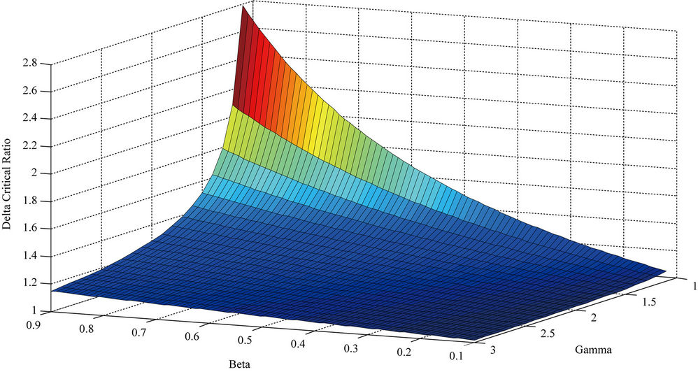
3.3. Effects of Beta on Delta Critical Ratios
Figure 3 depicts how that the delta critical ratios are greater for high values of beta and low values of gamma. The delta critical ratios are about equally affected by gamma as they are beta for our range considered. Given large values of gamma, beta has little effect on the delta critical ratio. For small values of gamma, beta has a great effect on delta critical ratios. Conversely, gamma effects delta critical more greatly for larger values of beta, and less for lower values of beta. Figure 3 suggests that for materials that have low heat retention, the effect of heat dissipation greatly affects the heat that is requiring for heat explosion. For a material that has high heat retention, it is not as important to consider the effects of heat dissipation as the effect on the temperature at which heat explosion occurs.
Considering a situation where the factor of heat removal is considered constant, if the heat removal factor is low, then the temperature at which heat explosions occurs does not vary in respect to the heat retention of the material. For high heat removal factors, a small heat retention property in the material used will maximize the temperature at which heat explosion will occur.
4. Conclusions
This paper presents a study in the causes of heat explosion through a mathematical approach. The simplified approach to modeling heat explosion represents a direct
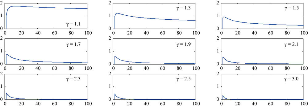
Figure 1. Each subplot illustrates the delta values for Tm between 0 and 100 at a different gamma value. The peak of each plot represents delta critical.
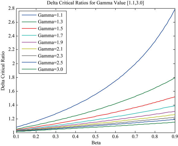
Figure 2. Delta critical ratios are displayed as beta ranges from 0.1 to 0.9. Each line reflects a different gamma value. These values are listed in the legend.
comparison between the effects of heat removal and the heat retention of the material. A better understanding of the causes of heat explosion has been achieved, as well as identifying the relative effect of heat removal and heat retention.
The Cauchy problem setting has shown that the material’s heat retention rate is about an equivalent factor to the conditions relevant to heat removal. Considering a scenario of an airplane wing where the material property will be held constant due to weight limits, it is important to consider that heat removal will have an influence on the rate of heat explosion. This will allow a company to modify air flow about the wing in order to improve the heat removal rate, and thus increase the heat required for heat explosion to occur. Observing a scenario of a component of an engine block where the boundary conditions are held constant. That is when the heat removal coefficient is constant, changing the material to be more resistant to heat change will increase the total heat required to enter the system for heat explosion to occur. When a company is experiencing heat explosion in a constant heat removal setting, it is important to consider material changes that would require a greater heat before heat explosion occurs.
The ultimate goal of our work is to create a well understood and reliable model to predict thermal failure given parameters for both the loading conditions and material properties. To do this we need to account for the degree to which each parameter contributes to heat explosion phenomena. In order to do this the next step is to use a sensitivity analysis on each of the contributing parameters. In doing so the materials can be evaluated for each parameter and materials can be selected for engineering designs conscious of evading problems with thermal failure. We also have interest in developing an additional model to account for thermal failure parameters on the basis of Maxwell’s laws of heat conduction. We will then compare these results to those modeled with Fourier’s law to determine the more accurate and efficient model. Another previously mentioned goal of our work is to develop a well known physical meaning and dimensions to the material parameters that are derived and input into the model. All of these goals combine to create a well understood, consistent and accurate model to predict thermal failure and allow for considerations during the process of material selection and design.
5. Acknowledgements
We would like to give special thanks to Clemson University and especially the College of Engineering and Science. This project could not have been possible without the contribution of workspace, software licensing and overall support from the faculty.
REFERENCES
- P. P. Oldyrev, “Heating-Up Temperature and Failure of Plastics under Cyclic Deformation,” Mechanics of Polymers, Vol. 3, 1967, pp. 483-492.
- P. P. Oldyrev and V. P. Tamuz, “Change in Properties of Glass-Reinforced Plastic under Cyclic Tension-Compression,” Mechanics of Polymers, Vol. 5, 1967, pp. 864-872.
- P. H. Francis, “Thermo-Mechanical Effects in Elastic Wave Propagation: A Survey,” Journal of Sound and Vibration, Vol. 21, No. 2, 1972, pp. 181-192. doi:10.1016/0022-460X(72)90905-4
- D. Meinkohn, “Heat Explosion Theory and Vibrational Heating of Polymers,” International Journal of Heat and Mass Transfer, Vol. 25, No. 4, 1981, pp. 645-648. doi:10.1016/0017-9310(81)90008-9
- I. Viktorova, J. V. Suvorova and A. E. Osokin, “Self- Heating of Inelastic Composites under Cyclic Deformation,” Izvestiya AN USSR Mechanics of Solids, Vol. 19, No. 1, 1984, pp. 99-105.
- I. Viktorova, “The Dependence of Heat Evaluation on Parameters of Cyclic Deformation Process,” Izvestiya AN USSR Mechanics of Solids, No. 4, 1981, pp. 110-114.
Appendix
Matlab Code 1—Computes Delta Critical Values and Plot Figure 1
%beta=0 gammas=[1.1,1.3,1.5,1.7,1.9,2.1,2.3,2.5,3.0];
for i=1:1:9 gamma=gammas(1,i);
for k=2:1:1002 T_m(1,k)=k;
fun20= @(n) (1./(sqrt(1-n.^(1+gamma))));
z1=quad(fun20,1/k,1);
Eq20(1,k)=((1+gamma)/2)*((k^((1-gamma)/2))*z1)^2;
subplot(3,3,i)
plot(T_m,Eq20)
axis ([0 1010 0 2])
MAX(1,i)=max(Eq20);
end end
Matlab Code 2—Computes Delta Critical Ratio Values and Plot Figures 2 and 3
gammas=[1.1:.1:3];
for m=1:1:20 gamma=gammas(1,m)
betas=linspace(0.1,0.9,80);
for j=1:1:80 beta=betas(1,j);
i=1;
spoint=1.1;
fpoint=.5;
epoint=51.1;
for k=spoint:fpoint:epoint %With beta T_m(1,i)=k;
fun21= @(T) (1./(sqrt(((k.^(1+gamma))-(T.^(1+gamma))) +(((beta*(1+gamma))./2).*(T-k).*(T+k-2)))));
z2=quad(fun21,1,k);
Eq21(1,i)=(z2^2)*((1+gamma)/2);
%Without beta T_m(1,i)=k;
fun20= @(n) (1./(sqrt(1-n.^(1+gamma))));
z1=quad(fun20,1/k,1);
Eq20(1,i)=((1+gamma)/2)*((k^((1-gamma)/2))*z1)^2;
i=i+1;
end
[Max21,T_mc1]=max(Eq21);
[Max20,T_mc2]=max(Eq20);
T_mc1=(T_mc1*fpoint)+spoint;
T_mc2=(T_mc2*fpoint)+spoint;
if T_mc1==T_mc2 T_mc(m,j)=T_mc1;
deltar(m,j)=Max21/Max20;
deltas(m,j)=Max21-Max20;
delta21(m,j)=Max21;
delta20(m,j)=Max20;
else error('T_mc values differ');
end end end plot(betas,deltar)
xlabel('Beta')
ylabel('Delta Critical Ratio')
title('Delta Critical Ratios for Gamma Value [1.1,3.0]')
legend('Gamma=1.1','Gamma=1.2','Gamma=1.3', 'Gamma=1.4','Gamma=1.5','Gamma=1.6','Gamma=1.7','Gamma=1.8','Gamma=1.9','Gamma=2.0','Gamma=2.1','Gamma=2.2','Gamma=2.3','Gamma=2.4','Gamma=2.5','Gamma=2.6','Gamma=2.7','Gamma=2.8','Gamma=2.9','Gamma=3.0','Location','NorthWest')
figure surf(betas,gammas,deltar)