Modern Economy
Vol.4 No.4(2013), Article ID:30756,12 pages DOI:10.4236/me.2013.44032
Dynamic Effect of Low-Cost Entry on the Conduct Parameter: An Early-Stage Analysis of Southwest Airlines and America West Airlines
Graduate School of Business, Kobe University, Kobe, Japan
Email: hidekim@panda.kobe-u.ac.jp
Copyright © 2013 Hideki Murakami. This is an open access article distributed under the Creative Commons Attribution License, which permits unrestricted use, distribution, and reproduction in any medium, provided the original work is properly cited.
Received January 8, 2013; revised February 14, 2013; accepted March 10, 2013
Keywords: Low-Cost Carrier (LCC); Entry; Dynamic Analysis; Conduct Parameter
ABSTRACT
The purpose of this research is to investigate the dynamic changes in the competition between air carriers by applying a revised conduct parameter method. We examine the cases of Southwest Airlines and America West Airlines due to the availability of data. Our interests are in what fashion a low-cost carrier entered the market, how the rival reacted, and whether the fashions of competition between two types of air carrier remained stable as time passed. Our empirical results show that the fashions of competition fell between Cournot and “P = MC” competition, and competitive fashions were sometimes stable but sometimes not.
1. Introduction
As the market share of the low-cost carriers (LCCs) in the airline industry has grown to about 30% of the total revenue passengers worldwide, many academic studies on the issues of LCCs have been published. Among these studies, not a few have focused on the effect of an LCC’s entry on airfares and welfare issues, but only a little attention has been paid to the fashions of competition between LCCs and full-service airlines (FSAs) using the conduct parameter method (CPM).
Other than the studies on the application of CPM to the airline industry, there have been many studies on the economic impact of the entry of the US LCCs (especially Southwest Airlines) into the air transportation markets. Morrison and Winston’s study [1] empirically showed that Southwest Airlines forces its competitors to reduce their fares [1, pp. 132-156]. [2,3] have measured the airfare-reduction effect of LCC entry in the primary and adjacent markets by incorporating LCC dummy variables in their econometric work. [4] empirically analyzed the US domestic air markets that include a number of LCCs and found that Southwest Airlines, other LCCs, and the market share of LCCs had statistically significant effects on the decrease in carriers’ airfares.
The recent contributions to the study of inter-firm rivalry among air carriers are as follows [5,6]: studied the effects of LCC entries on the incumbents’ responses. [7] incorporated duopolistic inter-firm rivalry explicitly into their LCCs vs. FSAs competition study, as well as incorporating the effect of pricing behavior of an unregulated-monopoly airport on the downstream competition between LCCs and FSAs. [8] found that the service differentiation between FSAs and LCCs leads to the cartelized behavior of FSAs.
In analyses that used CPM [9-11], empirically estimated the conduct parameters of airline industries in the United States (the first two of three studies), Spain (the fourth study), and Japan. The earliest contributions of applying CPM to the airline industry are those of [12-14], who analyzed the inter-firm rivalry between FSAs.
Our research will also apply the newly revised CPM to the analysis of the competition between LCCs and FSAs, and the distinguishing feature of our analysis is that we focus on the dynamic aspects of competitions. We will discuss the basic concept of CPM and also review the pros and cons of this method for analyzing competition in the next section, highlighting the studies of [15,16]. In Section 3, we will show how to overcome the drawbacks of CPM by quoting the methodology of [16]. In Section 4, we construct an econometric model of demand and the pseudo-supply equation system to derive the conduct parameters. In Section 5, we will show the dataset for our empirical analysis. Section 6 demonstrates the dynamic change in the conduct parameter after the entry of Southwest Airlines, and we discuss the results. In Section 7 (the final section), we will demonstrate the contributions of our research and discuss the implications of industrial policy. Finally, we will mention the limitations of this study, which will guide us in improving our analyses in the future.
2. CPM and Dynamic Competition
Reviewing the pertinent literature, we find that there have been two ways to estimate the conduct parameter. One method was proposed by [12-14], who estimated the non-liner pseudo-supply equation and the demand equation jointly. The alternative method was proposed by [17,18], who estimated the linear inverse demand and the pseudo-supply equation jointly. The major difference between the two methods is that the former method directly estimates the conduct parameter, while the latter method derives it indirectly from the parameters of output variables in the inverse demand and the pseudo-supply equations.
In a recent analysis of the estimation of market power using CPM [9], pointed out that in a static environment, the notions of expectation and conjectural variation are not well defined. For example, if we start our analysis by modeling a one-shot Cournot competition and try to estimate the conjectural variation by CPM, we face the problem that we cannot describe a firm’s response or any dynamic change in the firm’s behavior. As [19] stated, “The estimated parameters tell us about airfareand quantity-setting behavior; if the estimated ‘conjectures’ are constant over time, and if breakdowns in the collusive arrangements are infrequent, we can safely interpret the parameters as measuring the average collusiveness of conduct” [19, p. 129]. Also, [15] pointed out, “CPM estimates of market power can be seriously misleading. In fact, the conduct parameter need not even be positively correlated with the true measure of the elasticity-adjusted price-cost margin, so that some markets are deemed more competitive than a Cournot equilibrium even though the price-cost margin approximates the fully collusive jointprofit maximizing price-cost margin” [15, p. 299].
CPM is also criticized by [20-22]. We can classify the pitfalls of CPM into two parts. The first one is the problem with the link between theoretical and empirical methods. [20] pointed out that the estimated conduct parameter can represent the theoretically derived conduct parameter only under a specific information assumption. We repeat [15]’s critique of CPM that, since it assumes a static model, CPM does not explain the reaction of firms or the incentive compatibility constraint that indicates why a firm stays in a collusion situation or deviates from it. Therefore, CPM may yield an inconsistent estimator of the market power when firms are engaged in tacit collusion in a dynamic competition. The second type of pitfall is the problem with the functional form: earlier literature such as the studies by [19,23] pointed out that the estimation of the conduct parameter varies widely depending on the functional form. [22,24] studied the conduct parameter of the electricity market in Britain (the former) and California (the latter) using the directly measured and the estimated marginal costs, and concluded that the latter method (NEIO method) overstated the market power.
Taking these critics’ statements into account [9], nonetheless stressed the usefulness of conjectural variation. They insisted, following [13,14], that “one can view the conjectural variation as a parameter of market conduct that can capture the whole range of market performance, from perfect competition to monopolistic behavior, rather than taking it as an indicator for the firm’s expectation” [9, p. 234]. [10] also computed the conduct parameters of Spanish air markets by estimating the demand and pseudosupply equation system using semi-annual (summer and winter) data of the years 2000 and 2001 by three stage least square methods (3SLS), not stressing the problem with the dynamic features of conduct parameters but regarding conduct parameters as the set of static equilibria [10, pp. 388-395].
[22] summarized the conjectural variation model to state that it is a proxy for a dynamic model, and the folk theorem tells us that a range of conducts are Nash equilibria in a dynamic game. Therefore, one can view the conjectural variation not as an estimate of a theoretical model, but as a measure of the elasticity-adjusted Lerner index, measuring the static-equivalent level of an Industry’s competitiveness. Provided the technique yields accurate estimates of the elasticity-adjusted Lerner index, it is a useful exercise.
Other research such as the studies by [25,26] pointed out that the estimates of conjectural variation are robust across functional form. The most recent remedy for CPM is that by [16], which tried to answer the critique of [15]. In summary, the estimate of conduct parameter could overstate, understate, or be close to the theoretical value.
The next section focuses on reviewing the critique by [15] and the remedy proposed by [16].
3. The Application of CPM to Deduce the Degree of Competition: Critique by Corts and Counterproposal by Puller
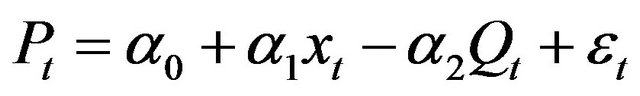
Corts’ article [6] assumed that we must estimate the following linear demand and supply system using timeseries data (t denotes time period):
 (1)
(1)
 (2)
(2)
In Equation (1),  is a vector of demand shifters,
  is firm i’s output, and
  (N is the number of symmetric firms). Thus, Equation (1) represents an inverse demand function, with
  being the random disturbance. In Equation (2),
  is the vector of cost shifters, and thus Equation (2) represents a pseudo-supply function, with
  being the random disturbance term. The 2SLS estimator of
  is as follows:
The asymptotic estimator of 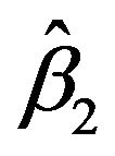 which can be derived by 2SLS, is
 , where
  is the parameter obtained by regressing
  on
on . Let
. Let  be the asymptotically consistent estimator of conduct parameter, such that
 (3)
(3)
We see that the estimated conduct parameter is a function of only the demand parameters and , the responsiveness of equilibrium quantity to the demand shifter. Theoretically, the conduct parameter measures something having to do with the slope of the supply relation. Assuming a firm’s optimum supply on the pseudo-supply curve is linear in
 , i.e.,
 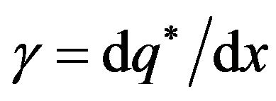 , then the estimated conduct parameter measures the slope of the pricecost margin with respect to demand driven fluctuations in quantity, as follows:
 (4)
(4)
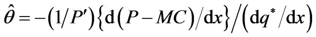
On the other hand, the conduct parameter, which is theoretically derived from the first-order condition (the so-called “as-if” conjectural variation), is depicted as a static form, as follows:
 (5)
(5)
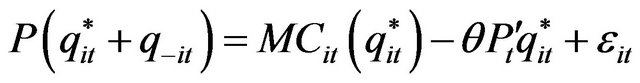
Therefore, Corts proposed that for any underlying supply process generating , the estimated conduct parameter would accurately measure market power
 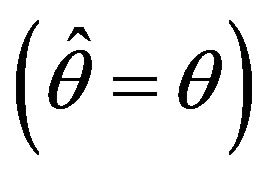 if and only if
 (6)
(6)
Otherwise, the estimated theta is not a consistent estimator of . Therefore, the essence of Corts’ critique is that the conduct parameter derived from CPM does not capture any dynamic aspect, even in the case of a dataset that has a time-series dimension.
[16] reviewed Corts’ critique and suggested the following theoretical model to obtain a consistent estimate of  in a dynamic game. Note that the following discussion is taken from [16, pp. 1497-1500]. In this model, a firm maximizes the joint profit so that no firm will deviate from collusion at t in the infinite game (and also in a finite game with many repetitions), as follows:
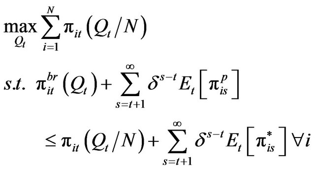 (7)
(7)
where 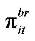 is the one-shot game profit of a deviated firm,
 ![]() is the discount factor,
is the discount factor,  is the firm’s optimal profit under collusion,
 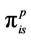 is the firm’s profit after it has deviated, and
  is the expectation. The first-order condition with respect to
  yielding the condition that each firm in a collusive regime satisfies is as follows:
 (8)
(8)
where  is the Lagrange multiplier on the incentive compatibility constraint and
 ![]() is the conduct parameter. According to [16], Equation (8) has a simple interpretation. In a collusive equilibrium, the firm internalizes the effect of price changes on the revenue for all firms’ inframarginal output
is the conduct parameter. According to [16], Equation (8) has a simple interpretation. In a collusive equilibrium, the firm internalizes the effect of price changes on the revenue for all firms’ inframarginal output . When the incentive compatibility constraint is not binding
 , the last term will be zero and we get the firm-level first-order condition for joint monopoly pricing. When the constraint binds, the joint output must rise and the price must fall, so no firm will deviate, i.e., firms collude between the monopoly and Cournot levels. It is apparent that Equation (8) can explain the dynamic situation as well as the situation where firms play a one-shot game.
In the one-shot game, the last term on the right-hand side of Equation (8) is zero, since  . This equation captures the following three common oligopoly models:
H1: “P=MC”: 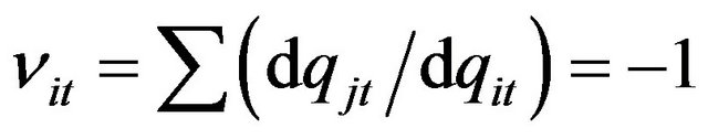 and
and  .
.
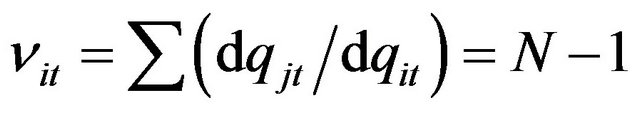
H2: Cournot: 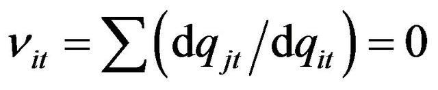 and
and .
.
H3: Efficient tacit collusion:
 and
and  where
where
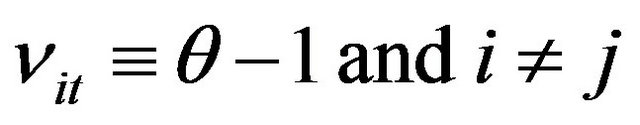 .
.
If we regard the last term on the left-hand side of Equation (8) as a random disturbance of an econometric model, we can rewrite Equation (9) as follows:
 (9)
(9)
If  is non-zero and correlated with
  , the conduct parameter to be estimated is biased and inconsistent due to the simultaneous-equation bias. This problem can be avoided by using two-stage least squares if there is no heteroskedasticity. However, we have another problem to solve.
The last term in Equation (9) is equal across firms in the collusive regime for a given period. Based on this observation [16], stated that although one does not have the data on the last term in Equation (9), this term can be conditioned out by including a time fixed effect. Moreover, as discussed above, if firms are playing a static game, this term is zero, so Equation (9) can be generalized to both static and dynamic pricing, and it yields the consistent estimator of . The important point is that the conduct parameter in our analysis does not capture the reaction behavior such as Stackelberg competition, but it does demonstrate the series of “degree of market power” in one-shot games after an LCC’s entry. In addition, as will be shown in Section 4, our dataset is made up of the series of yearly sample observations, and each year’s estimate means the average Nash equilibria of a number of competitions performed in the year. The next section shows the structural pseudo-supply and demand model incorporating time fixed effect dummy variables.
4. Structural Equation for Deriving Dynamic Change in the Conduct Parameter
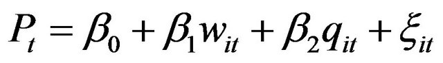
The empirical model to be estimated is the following simultaneous equation system consisting of the linear inverse-demand and the pseudo-supply equations, which follow the reports of [17,18] that were discussed in [15]:
(Inverse demand)
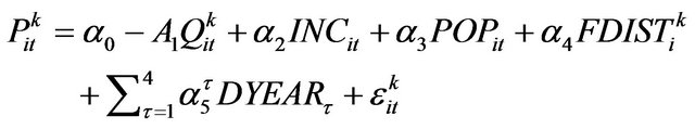
 (10)
(10)
where
(pseudo-supply)
 (11)
(11)
where
where 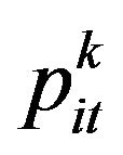 is the year-average airfare of carrier
  at route
  in year
  ,
,  is the number of passengers carried by carrier
  at route i in year
  ,
,  is the population-weighted average per-capita income of route i’s origin and destination areas in year
  ,
,  is the arithmetic average population of route i’s origin and destination areas in year t,
  is the distance flown by carrier k at route i1,
  is the route marginal cost of carrier k at route i in year t,
  is the Herfindahl index of route i in year t, and
  and
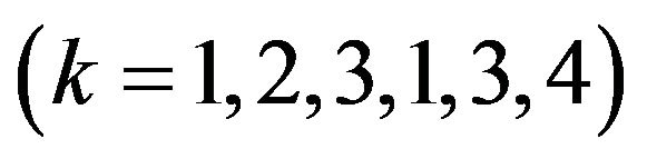
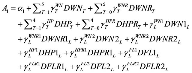
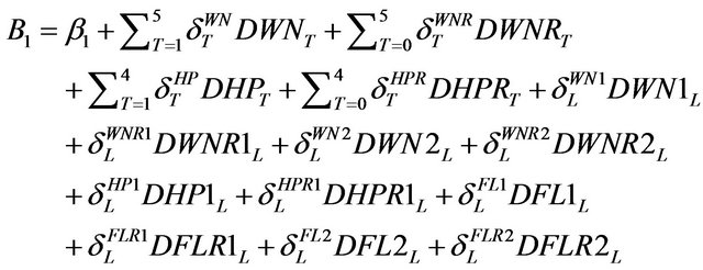
and  are the random disturbance terms. All the other variables starting with D are binary variables, and A₁ and B₁ denote the sets of parameter dummy variables introduced to the output variable of each demand and pseudo-supply equation. The explanations of these dummy variables are shown in Table 1.
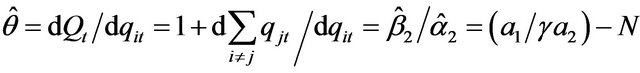
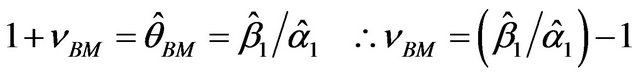
All these dummy variables are introduced as “parameter dummy variables” so as to compute the dynamic change in conduct parameters. Recalling Equation (4) in the last section, we can derive the conduct parameter of the benchmark carriers  . The benchmark carriers are FSAs that did not compete with LCC(s) for the period from 1997 to 2000 in their operating routes (for example, the case of the competition between AA and UA in a certain route). This is shown in the following equation:
 (12)
(12)
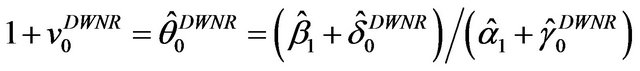
This means the conduct parameter is computed by dividing the estimated parameter of the output variable in the pseudo-supply equation by that of the output variable in the inverse demand equation, and this is a consistent estimator of the conduct parameter by introducing the time fixed effect dummy variables  . Similarly, the conduct parameter of Southwest’s rival in the pre-entry year is computed as follows:
 (13)
(13)
The image of this computation is shown in Figure 1.
Comparing Equation (12) with Equation (13), it is apparent that the angles of demand and pseudo-supply curves are different, although those of intercepts are the same. Assume X is the “benchmarking” demand and pseudo-supply equilibrium, and Y is the demand and pseudo-supply equilibrium that Southwest’s rivals had reached before Southwest Airlines entered the market. The conduct parameters that are computed from X and Y will be different from each other. We will do the same
Table 1. Explanations of binary variables.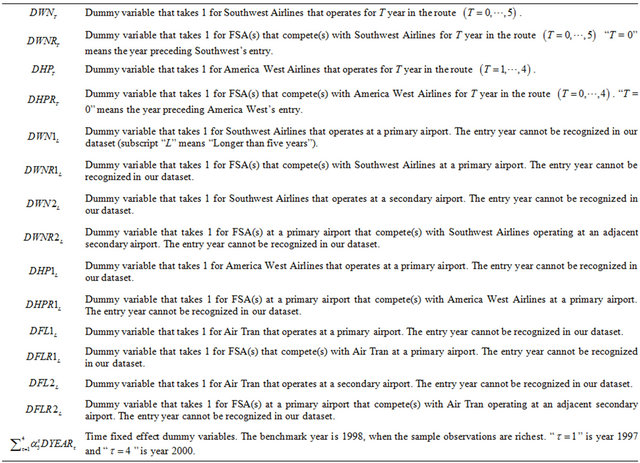
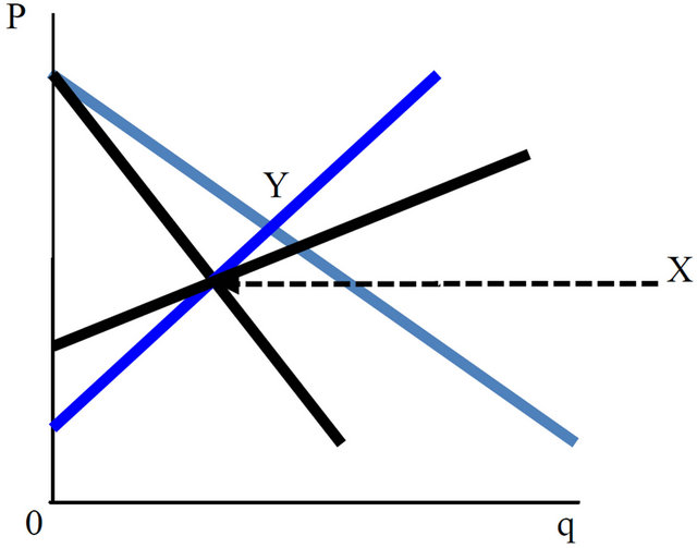
Figure 1. Graphical explanation of Equation (13).
computation for all the cases of the carrier dummy variables. The dummy variables and methods of computation are shown in Table 2.
Since the thetas in the right columns of Table 2 contain carriers’ own behavior (that is,  ), we need to deduce one i order to derive v, which stands for the sum of other carriers’ (j’s) reactions to carrier i’s behavior. One feature of the structural model is that we have information about the marginal cost. We used the route-specific marginal cost, which can be empirically derived, a method that was used in [11,12,14]. In addition, as one of the proxies of the marginal cost, we also used “distance flown by carriers”, since this proxy was used in recent reports such as that by [10]. In addition, following the standard literature on airline costs, we assumed that economies of density exists.
To estimate this structural model, we had to determine which method of estimation would best suit our purposes. Theoretically, price and quantity are both endogenous, so it is natural to estimate this equation system by 2SLS. The 2SLS method is, like OLS, efficient when the random disturbance follows normal distribution; however, if we recognize the heteroskedastic distribution of random disturbance, 3SLS is better than 2SLS in terms of estimation. To diagnose the heteroskedasticity, we performed the White-Kornker test for the demand and the pseudosupply equations. The test results were that for the demand equation ![]() and for the pseudo-
and for the pseudo-
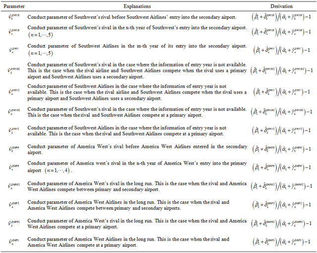
Table 2. Computing method to derive a carrier-specific conduct parameter.
supply equation ![]() . These two values are large enough to allow us to reject the null hypothesis that we have no heteroskedasticity at the 1% level. Therefore, we used 3SLS for our estimation method. We used alternative methods such as iterative 3SLS or 2SLS, each of which is more efficient than 2SLS under heteroskedasticity.
. These two values are large enough to allow us to reject the null hypothesis that we have no heteroskedasticity at the 1% level. Therefore, we used 3SLS for our estimation method. We used alternative methods such as iterative 3SLS or 2SLS, each of which is more efficient than 2SLS under heteroskedasticity.
5. The Data
As in our first study of this subject, we collected operational data observations from DB1A, which included the available US domestic flight data for carriers that had 10% market share in duopoly markets. We omitted the data of carriers with less than 10% market share in duopoly markets, or 5% share in triopoly markets or markets served by more carriers. Carriers whose codes are not reported in DB1A (reported as XX) were also omitted, but, for example, a triopoly market with one XX carrier was not regarded as a duopoly market, since the XX carrier probably had competitive effects on the other carriers in that market. The flight data are outbound and non-connecting routes from the seven largest US airports and their regions: New York/Newark area, (JFK, LaGuardia, Newark), Washington, DC, area (Ronald Reagan (National), Dulles, Baltimore), Chicago area (O’Hare and Midway), Atlanta/Hartsfield area, Dallas/ Fort Worth area (DFW and Love Field), and Los Angeles.
The cost and input price data are from the Air Carrier Financial Reports, Form 41 Financial Data. Income and population data are from the Regional Accounts Data, Bureau of Economic Analysis. We used the Primary Metropolitan Statistical Area data (PMSA, an urbanized county or set of counties that have strong social and economic links to neighboring communities) for each city.
We used data from 199 city-pairs that are duopoly markets and 166 triopoly markets, which gave us 894 sample observations. The time-series dimension starts in 1996 and ends in the year 2000. We did not extend the time dimension beyond year 2000, because we would have had to remove the effect of the “9 - 11” terrorist attack in 2001. The descriptive statistics used for the analyses of this chapter are shown in Table 3.
6. Empirical Results of the Conduct Parameter
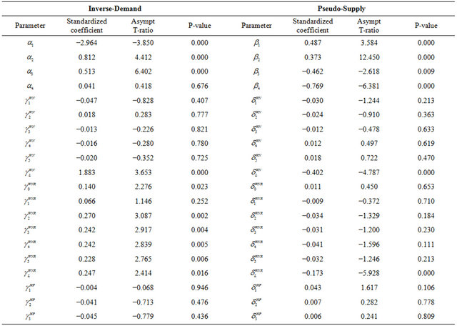
Competitions between LCCs and FSAs can be regarded as the competition with differentiated products or services that air carriers offer. However, although we admit that we may need the discussion from this “product-differentiation” viewpoint, we will focus on the discussions of the price-quantity issues to prevent our discussions from being vague. The detailed estimated results of Equations (11) and (12) are shown in Table 4 in Appendix. Figures 2 and 3 graphically show the dynamic changes in conduct parameters.
Overall, for both the case of Southwest Airlines and that of America West Airlines, in the single-year time span, carriers competed between the Cournot and the competitive level (that is,  distributes between zero and −1). Southwest Airlines’ conduct parameter is lower by 14% than those of the incumbent(s), and this means the incumbents reacted very competitively against Southwest Airlines’ entry. The incumbents’ conduct parameters dropped by 6.3% after Southwest Airlines entered, so it appears that Southwest Airlines also reacted more competitively than did other carriers that had operated before Southwest’s entry.
The case of America West Airlines is a little different from that of Southwest Airlines, except for the long-run result. Unlike Southwest Airlines, America West Airlines seems not to have carefully targeted which markets to enter: sometimes it entered markets where another LCC had already entered2. For example, America West entered the Chicago-Sacramento market in 1999, where Southwest Airlines and United Airlines were already competing.
Since competitions had already started in that market, Southwest Airlines and other incumbents were reacted by implementing tough strategies, even though America West’s market share in the beginning was small. The reason for the blue wavy line, which shows the reactions of Southwest and United Airlines, did not drop after America West Airlines entered is that these incumbent carriers including Southwest Airlines had already started competition before America West Airlines entered the market. In the fourth year of America West Airline’s operation in this market, when its market share increased, its rivals reacted even more competitively than they had in the former years.
In the case where we cannot identify when LCCs entered (i.e., in the long run), the incumbent(s)’ conduct parameter drops by 34% from the pre-entry level, and Southwest’s conduct parameter drops by 48.7%. Therefore, in the case of Southwest Airlines, the competition seems to last and become fierce after more than five years have passed. This is also true for the case of America West Airlines.
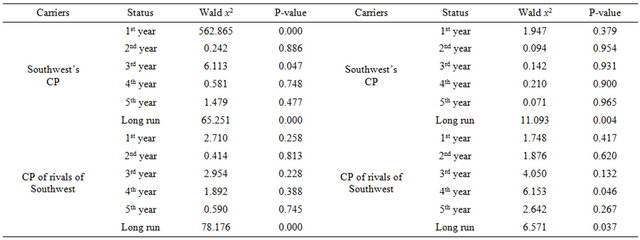
Our next goal was to determine whether the competitions between LCCs and FSAs are a series of “P = MC” competitions or a Cournot game in terms of statistics. To do this, we tested the hypotheses that the conduct parameters are −1 (the case of “P = MC” competition) and zero (Cournot case), while the parameters of entry-year time fixed effect dummy variables are simultaneously zero for “P = MC” competitions and Cournot cases. Table 5 shows the results of these joint tests of the two hypotheses for Southwest Airlines, and Table 6 shows the results for America West Airlines.
According to Tables 5 and 6, we can reject the hypothesis that a carrier performs Cournot competitions for the first year and the third year of Southwest Airline’s entry and the cases where competitions last for more than five years by carrying out the Wald  test with a degree of freedom equal to two.
Table 3. Descriptive statistics of continuous variables.
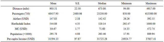
Note: Herfindahl index takes 1000 when monopoly.
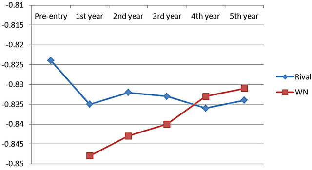
Figure 2. Dynamic changes in Southwest’s and its rivals’ conduct parameters.

Figure 3. Dynamic changes in America West’s and its rivals’ conduct parameters.
Table 5. The results of joint tests of hypothesis for Southwest Airlines.
Note: Left: test of Cournot hypothesis, Right: P = MC hypothesis.
Table 6. The results of joint tests of hypothesis for America West Airlines.
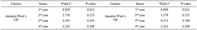
Note: Left: test of Cournot hypothesis, Right: P = MC hypothesis.
We cannot reject the hypothesis that the conduct parameter and the parameters of the entry-year time fixed effect dummy variable are equal to minus one at the 5% level for all the other cases of Southwest Airlines. As for other than the first year and the third year of Southwest’s entry, we cannot reject the hypothesis that the conduct parameter of Southwest Airlines is either minus one or zero. Considering these values of the conduct parameters, FSAs competed very fiercely, especially when Southwest Airlines entered the market, then softened competition in the second year, and again adopted a tough strategy in the third year. FSAs’ strategies were softened after the third year, and the fashion of competition fell between Cournot and “P = MC” competition.
Considering the conduct parameters of FSAs, Southwest’s fashion of competition fell between Cournot and “P = MC” competition. The data indicate those patterns had wide variation, except for the fourth year of Southwest’s entry: in the fourth year of entry, the competition was softer than in the previous years, and Southwest’s competition was of the Cournot type rather than the “P = MC” type.
As for the rivals of these two LCCs, Southwest’s rivals stayed at an in-between level, but America West’s rivals took a closer strategy to Cournot than to “P = MC” competition.
It appears the average value of America West’s conduct parameter is higher than that of Southwest Airlines, but there are no significant differences from a statistical viewpoint3.
When competitions lasted for more than five years for Southwest Airlines or four years for America West Airlines, it can be firmly stated that the patterns of competition were neither at the Cournot nor the “P = MC” competition level; that is, they were between the two. This result may have come from the fact that we have abundant sample observations for these cases, so the  value asymptotically became stable.
7. Concluding Remarks
This paper analyzed the dynamic change in the fashions of competition between Southwest Airlines and FSAs, and between America West Airlines and FSAs by using CPM. This method might have been a “dead end” method but for the proposals made by [16]. The methodological contribution of this paper is to re-vitalize CPM and apply Puller’s proposals for modeling the simultaneous equation system to deduce the fashions of dynamic competitions between FSAs and LCCs for the first time. The empirical contributions are that we were able to estimate the consistent conduct parameters for the analyses of dynamic competition and found the facts summarized in Tables 7 and 8.
The implication for the policy of the U.S. airline industry is that the competitions between LCCs and FSAs never reached the equilibrium state where social welfare is maximized (i.e., the “P = MC” level), even after 5 or more years. One possible explanation of this fact is that the market segments of FSAs were partly separated from those of LCCs, and both FSAs and LCCs had market power to increase their price-cost margins.
These situations may have taken place where either FSAs succeeded in differentiating their services against those of LCCs or vise-versa, and eventually the airlines differentiating services gained the power to be able to control their price-cost margins. There may be room for further discussion about whether government sectors have to intervene to remove these market powers or let the industry be “as-is” as long as consumers have several choices of carriers and behave on the basis of their willingness to pay.
Table 7. The fashion of dynamic competition between Southwest Airlines and its rivals.
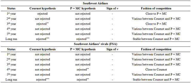
Note: that ***shows the hypothesis was rejected at 1%, **at 5%, and *at 10%, respectively.
Table 8. The fashion of dynamic competition between America West Airlines and its rivals.
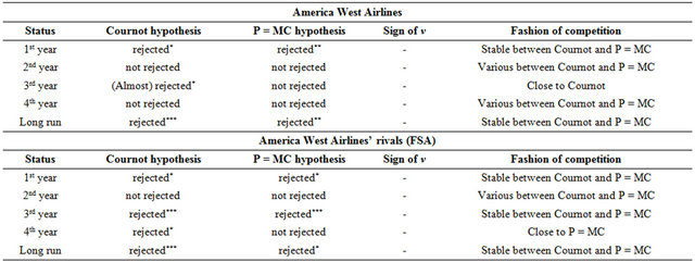
Note: that ***shows the hypothesis was rejected at 1%, **at 5%, and *at 10%, respectively.
Of course, our paper has limitations. One is that the data used here are “dated,” although we intended to avoid the effect of 9 - 11 terrorism and wars in the Middle East following 9 - 11. The second limitation is that we did not widen the range of our analyses to include other LCCs such as Air Tran and Jet Blue. This will be possible if we extend the time dimension of the dataset in future analyses. A third possible limitation is that we did not try to determine how the welfare changed over time in accordance with the change in the fashion of competitions, due to the limitation of the length of article. We will analyze these three issues in the future.
REFERENCES
- S. A. Morrison and C. Winston, “The Evolution of Airline Industry,” Brookings Institution, 1995.
- M. Dresner, J. S. C. Lin and R. Windle, “The Impact of Low-Cost Carriers on Airport and Route Competition,” Journal of Transport Economics and Policy, Vol. 30, No. 3, 1996, pp. 309-328.
- S. A. Morrison, “Actual, Adjacent, and Potential Competition: Estimating the Full Effect of Southwest Airlines,” Journal of Transport Economics and Policy, Vol. 35, No. 2, 2001, pp. 239-256.
- T. W. Vowles, “The Effect of Low Fare Air Carriers on Airfares in the US,” Journal of Transport Geography, Vol. 8, No. 2, 2000, pp. 121-128. doi:10.1016/S0966-6923(99)00033-2
- A. Goolsbee and C. Syverson, “How Do Incumbents Respond to the Threat of Entry? Evidence from the Major Airlines,” NBER Working Paper, 2005.
- A. V. M. Oliveira and C. Huse, “Localized Competitive Advantage and Price Reactions to Entry: Full-Service vs. Low-Cost Airlines in Recently Liberalized Emerging Markets,” Transportation Research Part E, Vol. 45, No. 2, 2009, pp. 307-320. doi:10.1016/j.tre.2008.09.003
- X. Fu, M. Lijesen and T. H. Oum, “An Analysis of Airport Pricing and Regulation in the Presence of Competition between Full Service Airlines and Low Cost Carriers,” Journal of Transport Economics and Policy, Vol. 40, No. 3, 2006, pp. 425-447.
- X. Fu, M. Dresner and T. H. Oum, “Effects of Transport Service Differentiation in the US Domestic Airline Market,” Transportation Research Part E, Vol. 47, No. 3, 2011, pp. 297-305. doi:10.1016/j.tre.2010.11.002
- T. Fischer and D. R. Kamerschen, “Price-Cost Margins in the US Airline Industry Using a Conjectural Variation Approach,” Journal of Transport Economics and Policy, Vol. 37, No. 2, 2003, pp. 227-259.
- X. Fageda, “Measuring Conduct and Cost Parameters in the Spanish Airline Market,” Review of Industrial Organization, Vol. 28, No. 4, 2006, pp. 279-399. doi:10.1007/s11151-006-9104-x
- H. Murakami, “An Empirical Analysis of Inter-Firm Rivalry between Japanese Full-Service and Low-Cost Carriers,” Pacific Economic Review, Vol. 16, No. 1, 2011, pp. 103-119. doi:10.1111/j.1468-0106.2010.00537.x
- J. A. Brander and A. Zhang, “Market Conduct in the Airline Industry: An Empirical Investigation,” RAND Journal of Economics, Vol. 21, No. 4, 1990, pp. 567-583.
- J. A. Brander and A. Zhang, “Dynamic Oligopoly Behavior in the Airline Industry,” International Journal of Industrial Organization, Vol. 11, No. 3, 1993, pp. 407- 435. doi:10.1016/0167-7187(93)90017-7
- T. H. Oum, A. Zhang and Y. Zhang, “Inter-Firm Rivalry and Firm-Specific Price Elasticities in the Deregulated Airline Markets,” Journal of Transport Economics and Policy, Vol. 27, No. 2, 1993, pp. 171-192.
- K. S. Corts, “Conduct Parameters and the Measurement of Market Power,” Journal of Econometrics, Vol. 88, No. 2, 1999, pp. 227-250. doi:10.1016/S0304-4076(98)00028-1
- S. L. Puller, “Estimation of Competitive Conduct When Firms Efficiency Colluding: Addressing the Corts Critique,” Applied Economics Letters, Vol. 16, No. 15, 2009, pp. 1497-1500. doi:10.1080/13504850701578900
- G. Iwata, “Measurement of Conjectural Variation Oligopoly”, Econometrica, Vol. 42, No. 5, 1974, pp. 947- 966. doi:10.2307/1913800
- T. Bresnahan, “Duopoly Models with Consistent Conjectures,” American Economic Review, Vol. 71, No. 5, 1981, pp. 934-945.
- T. Bresnahan, “Empirical Studies of Industries with Market Power,” In: R. Schmalansee and R. Willig, Eds., The Handbook of Industrial Organization, Vol. II, Elsevier, Amsterdam, 1989, pp. 1011-1057.
- T. Lindh, “The Inconsistency of Consistent Conjectures: Coming Back to Cournot,” Journal of Economic Behavior and Organization, Vol. 18, No. 1, 1992, pp. 69-90. doi:10.1016/0167-2681(92)90053-E
- P. C. Reiss and F. A. Wolak, “Structural Econometrics Modeling: Rationales and Examples from Industrial Organization,” In J. J. Heckman and E. E. Leaner, Eds., Handbook of Econometrics, Vol. 6, Part 1, Elsevier, Amsterdam, 2007, pp. 4277-4415.
- D. W. Kim and C. R. Knittel, “Biases in Static Oligopoly Models: Evidence from the California Electricity Market,” Journal of Industrial Economics, Vol. 54, No. 4, 2006, pp. 451-470. doi:10.1111/j.1467-6451.2006.00296.x
- L. J. Lau, “On Identifying the Degree of Competitiveness from Industry Price and Output Data,” Economic Letters, Vol. 10, No. 1-2, 1982, pp. 93-99. doi:10.1016/0165-1765(82)90122-7
- C. D. Wolfram, “Measuring Duopoly Power in the British Electricity Spot Market,” American Economic Review, Vol. 89, No. 4, 1999, pp. 805-826. doi:10.1257/aer.89.4.805
- K. Clay and W. Troeskin, “Further Test of Static Oligopoly Models: Whiskey, 1882-1898,” Journal of Industrial Economics, Vol. 51, No. 2, 2003, pp. 151-166. doi:10.1111/1467-6451.00196
- D. Genesove and W. Mullin, “Testing Static Oligopoly Models: Conduct and Cost in the Sugar Industry, 1890- 1914,” RAND Journal of Economics, Vol. 29, No. 2, 1994, pp. 355-377.
Appendix
Table 4. Demand and Pseudo-supply equations to derive conduct parameters.
NOTES
1The distance flown by each carrier is not equal across carriers, since LCCs flown from a secondary airport take different flight courses than do FSAs flown from a primary airport, though the difference of distance may be small.

2Such a case rarely happens to Southwest Airlines. It carefully targets the monopoly or joint-monopoly market from which it potentially can make abundant profits.

3We tested the null hypothesis that the conduct parameters of Southwest Airlines and those of America West Airlines are equal ( , τ = 1, ∙∙∙,4) by the Wald test. The x2 statistics with degree of freedom equal to one are 0.170, 0.0001, 0.021, and 0.004, respectively. Since the x2 statistics at the 5% level of significance with d.o. f = 1 is 3.84, we cannot reject the null hypothesis.