Energy and Power Engineering
Vol. 5 No. 4 (2013) , Article ID: 33279 , 11 pages DOI:10.4236/epe.2013.54034
Influence of Different Degrees of Complementarity of Solar and Hydro Energy Availability on the Performance of Hybrid Hydro PV Generating Plants
Instituto de Pesquisas Hidráulicas, Universidade Federal do Rio Grande do Sul, Porto Alegre, Brazil
Email: albeluco@iph.ufrgs.br
Copyright © 2013 Alexandre Beluco et al. This is an open access article distributed under the Creative Commons Attribution License, which permits unrestricted use, distribution, and reproduction in any medium, provided the original work is properly cited.
Received July 22, 2012; revised February 14, 2013; accepted February 21, 2013
Keywords: Hybrid Energy Plants; Energetic Complementarity; Performance Analysis; Computational Simulation; Software MATLAB
ABSTRACT
The complementarity of energy resources used in hybrid power generation can result in optimization of power capacity and reservation capabilities. This article is dedicated to the study of hybrid hydro PV systems. The goal is to establish the relationship between system performance and complementarity of energy resources. The study was carried out with computer simulations based on a method that uses ideal functions developed to describe the energy resources and determines a limit of performance. The results confirm expectations that performance, as measured by the total time of failure to meet demand, will be better as energy resources are complementary. Charts relating energy complementarity with failures are presented. The subsequent research work shall proceed to at least two different phases. In the first one, the method exposed in the present work shall be applied to real data and compared to the operation of existing hybrid plants. In the second phase, results shall be confronted with design parameters of hydro PV plants based on complementary resources. A next stage would be the enlargement of the method applied in this work for systems based on other energy resources, such as wind energy and ocean wave energy.
1. Introduction
Hybrid systems are an alternative technically and economically feasible for power generation in remote sites and in places where the power supply quality is compromised. Research on the performance of hybrid systems has enabled the use of energy resources that were not feasible in non-hybrids. The combination of dynamic characteristics of different energy resources has also allowed the overcoming of difficulties in meeting customer demand profiles.
The definition and the adjustment of strategies for the operation of hybrid systems are forcibly more complex than those for non-hybrid systems due to the complexity of the problems faced and the non-linear characteristics of some system components. The energy available from the sources involved may present some type of time or space complementarity or both and this complementarity may influence the sizing and the operation of the resulting power system.
The combination of hydroelectric and photovoltaic sources of energy in a generation system may reduce the cost of energy available in plants implemented in low hydroelectric potential sites for which main system interconnection costs prove prohibitive. Research on hybrid hydro PV plants can evaluate the use of water reservoirs and battery banks as alternatives for energy storage within a system and can also evaluate the advantages of generation from complementary energy sources.
A hybrid hydroelectric photovoltaic plant is a generation system based on a hydroelectric power plant and a set of photovoltaic modules operating together to satisfy the demand of an ensemble of consumer loads. The complementarity between the energy resources may then be beneficial for the sizing of components and for the operation of this type of system, possibly including various devices for energy storage. Reference [1] discusses this category of energetic system and even presents cost estimates for implementation and operation.
If the hydro and solar energy availabilities present time-complementary, the storage devices may be sized to optimize the operation of the hybrid system. The water reservoir may be sized for a shorter period, implying lower costs and lesser environmental impacts if the hydro generator operates with a PV generator and a battery bank provided there is a complementarity between the two energy sources. Reference [2] presents a dimensionless index, adopted also in the present article, that evaluates to the various degrees of complementarity.
This article applies the method proposed by the author [3] to relate the performance of hybrid systems with the energetic complementarity of energy resources, complementing the results presented for time complementarity. The proposed method is employed to study the relationship between the performance of hybrid systems and the time complementarity, energy complementarity and amplitude complementarity of energy resources.
The performance is evaluated by comparing the total time of failure in meeting consumer demand, measured by the failure index, F, as defined by Equation (1),
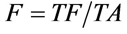 , (1)
, (1)
where TF is the total time of failure measured in the time interval considered in the analysis and TA é the total time considered in the analysis, usually equal to one year.
2. Simulation with the Method of the Theoretical Limit of Performance
The hybrid system under study, sketched in Figure 1, was simulated on computer with computational routines written with MATLAB [4] as described in [5].
The simulations adopt the pu system [6] to describe the physical quantities, where each quantity is divided by a reference value associated with the dimensions of each component of the system or with the reference values of available energy or demandThe operational strategy uses all the energy provided by the PV generator, operates the batteries in intermediate charge states; stores energy in the water reservoir and in the battery bank, their state of charge being managed as a function of the energy availability and demand while considering the possible energetic complementarity; and operates the hydro generator to address the consumer loads not attended by the PV generator, while considering the states of charge of the storage devices.
The operation of the hydro generator is obviously different from the usual operation of a hydroelectric power plant, as discussed for example by Reference [7], but it should be clear that a system like what is proposed in this work should be focused on better utilization of available power and simplicity of control.
The theoretical limit of performance [3] is defined as the upper limit for the performance of a power plant corresponding to the performance obtained with the “maximum availability” of the energy resource. This would be the maximum energy that could be available from a
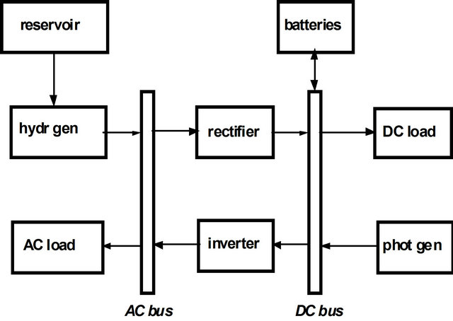
Figure 1. “Parallel” hydro PV hybrid power plant.
certain source if it were insensitive to random events typical of the environment and insensitive to periods of extreme energy scarcity or extreme availability.
The maximum and minimum average values for the total instantaneous available power to the PV generator were obtained from monthly data [8] for the region of Reference [2], considered in this study. The pu values of 0.67783 (corresponding to an incident solar radiation of 677.83W/m2) and of 0.37108 (corresponding to an incident solar radiation of 371.08 W/m2) are considered for the respective maximum and minimum instantaneous power available to the PV generator.
The simulated system is designed from the proportions between the total annual available and demanded energies (pad); the total annual available hydro and solar energies (psh); and the difference between the maximum and the minimum availabilities (pMm). For a constant demand profile the power required by the loads is considered equal to one. The available hydro and PV powers are defined as a function of the aforementioned proportions and present sinusoidal variations along the year.
Figure 2 shows the result of the simulation of a system with total complementarity and the battery bank sized for two days storage. The horizontal axis is time in years while in the vertical axis various functions are represented: to the left are the scales for the powers; to the right the state of charge of the batteries. The red line represents the graph shows the state of charge of the batteries (SOC). The blue, the hydroelectric power supplied (pH), the black stands for the maximum daily photovoltaic power (pP) and the green is the power consumed by the loads (pL). It can be seen that there are no shutoffs of the hydroelectric generator and no supply failures.
The complementarity index, k, is defined by Equation (2), where kt is the index for complementarity in time, ke is the index for energy complementarity and ka is the index for amplitude complementarity.
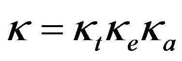 (2)
(2)
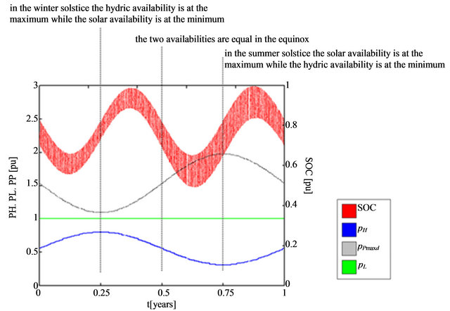
Figure 2. Results for a system with pad = 1.00, kt = 1.00; ke = 1.00 [psh = 1.00]; ka = 1.00 [pMm = 1.00] and kC = 1.00; with batteries with 2 days capacity with discharge to 40% and recharge to 100% of full capacity. Conventions: SOC: state of charge of batteries, pH: power from the hydro generator, pp: maximum daily power from the PV generator, pL: power supplied to the loads.
Equation (3) defines kt, where D is the day of the year for maximum availability, d é the day for minimum availability and the subscripts h and s distinguish hydropower and solar energy. Equation (4) defines ke, where E is the total annual energy. The definition of ka is more complex and requires a query to the Reference [2]. All rates of complementary vary between 0 and 1.
![]() (3)
(3)
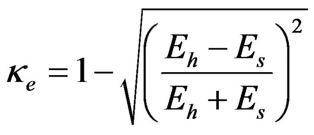 (4)
(4)
In the simulated system the annual energy available for consumption is equal to the demanded annual energy (pad = 1.00) and also the complementarity index is equal to one (kC = 1.00), which means perfect complementarity. Consequently, the time complementarity index kt, the energy complementarity index, ke, and the amplitude complementarity index, ka, are all equal to one.
The total annual solar energy available is equal to the total annual hydro energy available for the simulated system (psh = 1.00) and the differences between the maximum and the minimum solar energy availability and between the maximum and the minimum hydro energy availabilities are also equal (pMm = 1.00).
The days of maximum availability of solar and hydro energy, as well as their days of maximum and minimum hydro and solar energy availability, have lagged 180 days, leading to a perfect time complementarity (kt = 1.00). The ratio psh leads to a perfect energy complementarity (ke = 1.00) and the ratio pMm leads to a perfect amplitude complementarity (ka = 1.00).
This system was considered the “starting point” for the simulations, a pattern for easy comparisons with other results. The choice was made after a survey of different combinations of components and their importance for achieving the expected results.
The study of the effect of different degrees of complementarity on the performance of the energy system considered is based on the effects of the variations in the energy availability and of different combinations of installed power of hydro and of photovoltaic generator sets, in addition to the effects of the range of water discharges turning the hydroelectric generator.
3. Effect of Different Degrees of Complementarity in Time
The effect of variations in the time-complementarity index are illustrated in the results of reference [3], which presents the method and discusses the results of applying it in systems based on energy resources with different time lags. Figure 3 depicts the behavior of the failure index as a function of the time-complementarity index
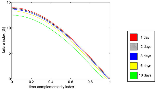
Figure 3. F as a function of kt for battery banks with 1, 2, 3, 5, 10 days capacity, for results of references [3,9].
for systems with 1, 2, 3, 5 and 10 days of batteries capacity for the results of references [3-9].
It is apparent that F is reduced with the increase in the time complementarity index and, consequently, with the improvement of the time complementarity characteristics of the energy availabilities. A lower capacity battery bank produces an upper shift of the curve due to a failure index increase while a bigger capacity bank produces a down shift towards smaller failure indexes.
It can be stated that the use of time-complementary energy resources contributes to the reduction of the failure index of a system, allowing the reduction of the size of the battery bank and the reduction of each generator installed power (as compared to equivalent one-generator systems of one type or the other).
Figure 3 shows how to improve the performance of a plant using intermediate or low time-complementarity. The increase in battery capacity leads to failure reduction but significant reductions involve high costs. The use of reservoirs may lead to greater reductions at costs varying with local conditions.
For example, a system with kt = 0.25 and somewhat less than 14% of failures, corresponding to approximately 50 days over a year, with a one season water reservoir may operate without supply failures. As another example, a system with kt = 0.50 and 8% of failures would require a water reservoir with a capacity of six months. A feasibility study should determine the appropriate size for the storage in either of these two cases, but reservoirs for a few weeks should significantly reduce failures.
4. Effect of Different Degrees of Energy Complementarity
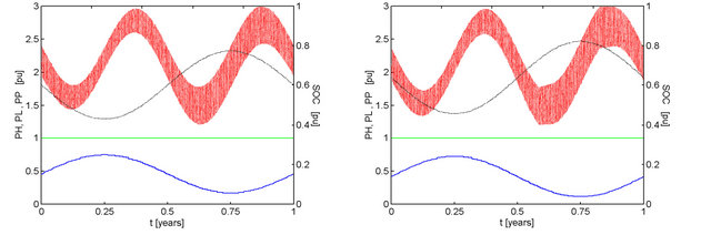
The effect of variations in the energy complementarity index is depicted in Figure 4. The graphs were made the same way as Figure 2. The values of ratio psh and index ke and the results for F appear listed in the legend of each result. Four results are shown, corresponding to the values of 1.43, 1.67, 0.70 and 0.60 for the ratio psh and the values of 0.8235 and 0.7500 for the energy complementtarity index. For reference, the system of Figure 2 has unity values for psh and ke.
The values of psh imply different average energy availabilities. For the first two results the photovoltaic energy supplied tends to increase while the supplied hydro power tends to decrease. Since the solar availability presents great daily and yearly variations, when its relative importance increases, so does the failure index. These variations cause corresponding, however subtly, amplified variations in the battery stored energy.
In the other two results the available photovoltaic power tends to decrease and the hydroelectric power tends to increase. As a growing fraction of the system energy tends to be “firm”, in view of its hydro origin, the failure index tends to decrease. It can be seen that from (c) to (d), chiefly in (d) an increase in the battery stored energy in the left side of the graph, as a consequence of the higher hydro availability.
It should, however, be emphasized that the variations of F are quite small and no changes are seen in the battery stored energy. In general, the variations in the energy-complementarity index cause variations in the fractions of the total energy supplied by each of the two generators. As the total available energy along the year remains constant, no important modifications occur either in the battery behavior or in the system performance.
It can be seen, however. that a bigger contribution by the hydroelectric power component leads to a failure free system while a bigger contribution of the energy of photovoltaic modules tends to require a bigger battery bank to avoid the failures. To some extent this limits the
 (a)
(a)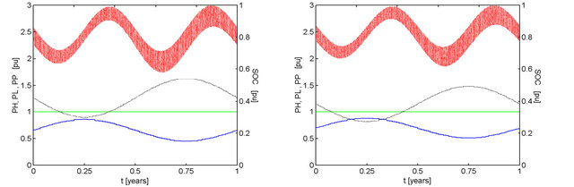 (b)
(b)
Figure 4. Effect of psh and ke on the performance of a system with kt = 1.00, ka = 1.00, with 2-day capacity battery bank discharged to 40% and recharged to 100% of maximum capacity. Conventions similar to those adopted in Figure 2. (a) psh = 1.43, ke = 0.8235, F = 0.0000; (b) psh = 1.67, ke = 0.7500, F = 0.0002; (c) psh = 0.70, ke = 0.8235, F = 0.0000; (d) psh = 0.60, ke = 0.7500, F = 0.0000.
applicability of hybrid hydroelectric photovoltaic generating plants to situations in which the hydroelectric power availability is insufficient.
These results show how a bigger contribution of the energy of photovoltaic modules implies a bigger energy storage capacity. The utilization of a reservoir may become easier to justify in the cases of near perfect timecomplementarity as the suitable effect of the energycomplementarity may be artificially obtained by the accumulation of hydraulic energy. A small increase in storage capacity may be sufficient to accommodate daily and seasonal variations in solar availability.
The small influence of the variations of energy complementarity on the failure index is quite evident. Failures remain under 0.40%, as can be seen from the results of Figure 4 and Reference [9], while the failures due to variations in the time complementarity index may be higher than 12%, as can be seen from the results of Figure 3, and the failures due to variations in the amplitude complementarity index are not greater than 7%, as can be seen from the results of Figure 5. These differences are certainly due to the method used.
5. Effects of Different Degrees of Amplitude Complementarity
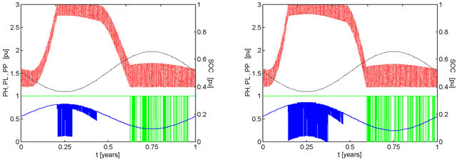
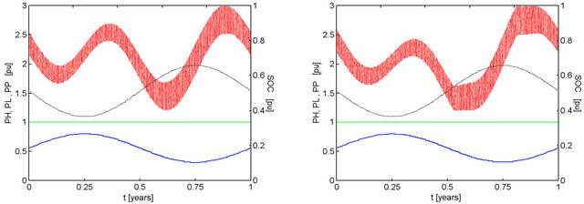
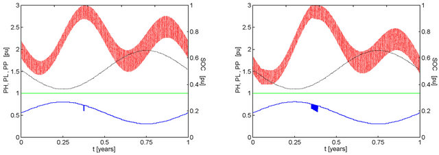
The effect of variations in the amplitude complementarity index is shown in Figures 6-9, summarized in Figure 5. The graphs were made the same way as Figure 2. The values of ratio pMm and index ka and the results for F appear listed in the legend of each result. Eight results are shown for the amplitude complementarity index values of 0.99, 0.96, 0.91, 0.84 (Figure 6), corresponding respectively to 1.11, 1.25, 1.43, 1.67 of ratio pMm, and 0.9878, 0.9412, 0.8448, 0.6923 (Figure 7), corresponding respectively to 0.90, 0.80, 0.70, 0.60 of ratio pMm. Other eight results are shown to detail the values of index ka close to unity, with 1.01, 1.02, 1.03, 1.04 (Figure 8) and with 0.99, 0.98, 0.97, 0.96 (Figure 9) for ratio pMm. For reference, the Figure 2 system has unity values for the proportion pMm and the index ka.
Importantly, the simulated systems with different ranges of energy availability, as they appear in different
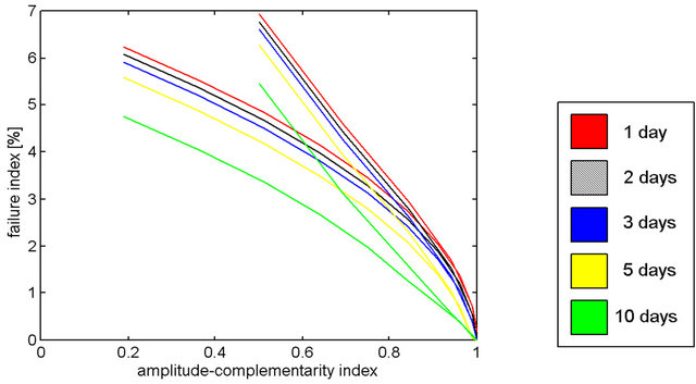
Figure 5. F as a function of ka for battery banks with 1, 2, 3, 5, 10 days capacity, for results of Figure 5 and reference [9].
 (a)
(a)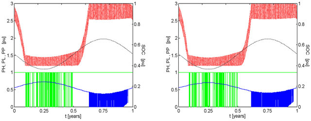 (b)
(b)
Figure 6. Effect of pMm and ka on the performance of a system with kt = 1.00, ke = 1.00, with 2-day capacity battery bank discharged to 40% and recharged to 100% of maximum capacity. Conventions similar to those adopted in Figure 2. (a) pMm = 1.11, ka = 0.9900, F = 0.0054; (b) pMm = 1.25, ka = 0.9600, F = 0.0121; (c) pMm = 1.43, ka = 0.9100, F = 0,0189; (d) pMm = 1.67, ka = 0.8400, F = 0.0259.
 (a)
(a)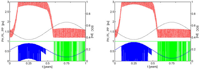 (b)
(b)
Figure 7. Effect of pMm and ka on the performance of a system with kt = 1.00, ke = 1.00, with 2-day capacity battery bank discharged to 40% and recharged to 100% of maximum capacity. Conventions similar to those adopted in Figure 2. (a) pMm = 0.90, ka = 0.9878, F = 0.0058; (b) pMm = 0.80, ka = 0.9412, F = 0.0153; (c) pMm = 0.70, ka = 0.8448, F = 0.0277; (d) pMm = 0.60, ka = 0.6923, F = 0.0443.
values for the ratio pMm, do not involve differences in the gap between the maximum availability (since kt = 1.00) or differences in energy availability (since ke = 1.00).
Different values of pMm do not affect the average hydro availability but represent the difference between its maximum and minimum values. In the four initially shown results (Figure 6) there is a reduction of hydro availability during the first semester so concentrating a growing number of failures in this period as well as keeping a correspondingly lower battery charge. As part of the hydro energy is transferred to the second semester, frequent reductions or shutdowns of the hydroelectric power will be observed.
In the subsequent four results (Figure 7), there is an increase in hydro energy in the first semester causing the reduction or shutting down of the hydroelectric power while failures and lower battery storage levels occur in the second semester. It is interesting to observe how the solar availability modulates the supplied hydroelectric power and the variations in battery stored energy.
Failures occur in these cases always at the end of the period of sunlight, by depletion of energy stored in batteries. This feature can be proven by way of lines in the graphs of these figures. Similarly, the hydroelectric generator is disconnected at the end of the period of sunlight, since the batteries are fully charged.
It shall be emphasized that the failure levels are intermediate between the values caused by time complementtarity variations (which go as high as 15% in the worse situations) and those due to energy complementarity variations (that are under 0.12%).
Failures in Figure 7 are somewhat larger than in Figure 6, but continue growing as complementarity decreases, as can be seen in Figure 5 in gray line, corresponding to batteries with 2 days of capacity. The greatest failures occurs in the second half because the minimum availability of solar energy occurs in the first half and this depletes the energy stored in batteries.
A reservoir with capacity of one week is sufficient to reduce failures to nearly zero for systems with more than
 (a)
(a)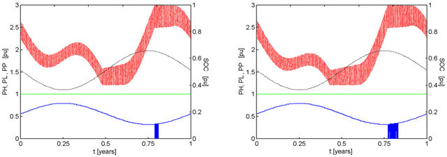 (b)
(b)
Figure 8. Effect of pMm and ka on the performance of a system with kt = 1.00, ke = 1.00, with 2-day capacity battery bank discharged to 40% and recharged to 100% of maximum capacity. Conventions similar to those adopted in Figure 2. (a) pMm = 1.01, ka = 0.9999, F = 0.0000; (b) pMm = 1.02, ka = 0.9996, F = 0.0006; (c) pMm = 1.03, ka = 0.9991, F = 0.0011; (d) pMm = 1.04, ka = 0.9984, F = 0.0017.
75% complementarity, which includes the results of Figure 6 and (a), (b) and (c) of Figure 7. Systems with less than 75% of complementarity will require larger reservoirs. The system of Figure 7(d) require a water reservoir with a capacity for fifteen days to not fail.
The use of real data, with daily variations of availability added to idealized values that were considered in the simulations, will change these results, requiring more storage capacity to compensate failures.
Obviously, it is possible to obtain storage capacity with other devices or other storage media. These water reservoirs above, with capacities of seven or fifteen days, could be substituted for example by banks of batteries. However, these banks would be extremely large compared to the reservoirs. Could also be used flywheels or air compressed or the system could be designed to include water or air heating.
There is a difference between the battery load variations over a year in Figure 2 and the results shown in Figures 6 and 7. In between there is a structural transition in the behavior of the energy stored in batteries. Figure 2 shows a variation that is due to the availability of hydropower and solar energy in equal measure in both semesters. Figures 6 and 7 show variations that are a consequence of the reduced availability of one of two energy resources in one or another half year.
Figure 8 details the transition in the behavior of the battery stored energy between the results of Figure 2 and those of Figure 6. It may be observed how the first peak of the curve collapses as a consequence of the increase of hydro availability in the first semester. In some results instances of shutdown of the hydroelectric generator occur approximately with the same timing as the peak of solar availability. The time span of these events is kept short by the subsequent reduction in solar availability.
Figure 9 details the transition in the behavior of the battery stored energy between the results of Figure 2 and those of Figure 7. Here the second peak is dissolved as a consequence of the increase in hydro power availability in the first semester. The hydroelectric generation is par-
 (a)
(a)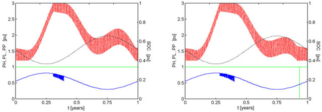 (b)
(b)
Figure 9. Effect of pMm and ka on the performance of a system with kt = 1.00, ke = 1.00, with 2-day capacity battery bank discharged to 40% and recharged to 100% of maximum capacity. Conventions similar to those adopted in Figure 2. (a) pMm = 0.99, ka = 0.9999, F = 0.0000; (b) pMm = 0.98, ka = 0.9996, F = 0.0002; (c) pMm = 0.97, ka = 0.9990, F = 0.0008; (d) pMm = 0.96, ka = 0.9983, F = 0.0014.
tial in some time intervals and not as frequent as in the results of the previous figure. The failures are less intense because the supplied photovoltaic power levels are quite high.
It is noticeable how the hydroelectric generator shutdown events grow frequent in the Figure 8 simulations, and how the failures and the partial generation events increase in Figure 9. Failures occur, initially, before and after the solar availability peak and, as the amplitudecomplementarity index departs from unity, they tend to fill even the peak time lapse.
In Figure 7(d), the disconnections of hydroelectric generator set (blue vertical lines) and failures to meet demand (green vertical lines) seem much more intense than it reveals the failure index of only 4.43%. Both, as well as the state of charge of batteries (red line), occur as a consequence of the characteristic of the availability characteristic of the solar energy, which prevails when the hydro availability is greater or less than the difference between the solar power available and consumer demand plus what can be stored in batteries.
These results show the sensitivity of the methodology to the variations of input data in a way similar to that discussed by the author [3], when the method was proposed and applied to the time complementarity.
Figure 5 depicts the behavior of the failure index as a function for the amplitude-complementarity index, with different sizes of battery banks, for the results of Figure 6 and of Reference [9]. A system with a smaller battery bank will present more failures and consequently an up-displaced curve. Conversely bigger battery banks reduce failures. If the supplied power is smaller than the available power, a small increase in installed power drives the battery charge levels up, near the upper limit.
The two sets of curves appearing in the chart of Figure 5 are associated with differences in the amplitude variation of energy resources. The set below, which in figure reaches a little over 6% failures, corresponds to the ratio pMm values smaller than one. The set higher, reaching almost 7% failures, corresponds to the ratio pMm values greater than one. If ratio pMm is greater than one, the range of variation of solar energy, mean the difference between its maximum and minimum values, will be larger, while if ratio pMm is less than one, the range of variation of hydropower will be higher.
In summary, then, the upper set in Figure 5 corresponds to systems with greater variation of solar energy, which have slightly larger values of failure index, while the lower set corresponds to systems with larger variations of hydroelectric power.
Situations similar to those in Figure 6 lead to reduced failure levels and may even eliminate failures altogether with the adoption of reservoirs allowing the transfer of energy from the second semester to the first semester of the subsequent year.
The same happens with the situations of Figure 7, except that the energy transfer should be from the first to the second semester. The values of the failure index lead to the proper sizing of the reservoirs, in general for a few weeks of operation.
These results were obtained from the application of the concept of theoretical limit of performance, as established by Reference [3]. Obviously, considering the actual data, the failures will be higher depending on the values of the complementarity index.
A failure reducing behavior as a function of the ka is to be expected as this index approaches its maximum value. Systems with pMm less than unity show failure slightly higher than those with pMm above unity. If a smaller battery bank is used the curve is shifted up. The reverse is verified for bigger batteries. The shape of these lines is obviously related to the definition of the amplitude complementarity index.
6. Discussion
The use of idealized data brought out various aspects of the performance of hybrid hydroelectric photovoltaic systems running on complementary energy resources. This procedure helps defining the applicability of the system and supports the sizing of its components.
A better time complementarity [3] is associated to smaller failure indexes. A reservoir may artificially improve time-complementarity having the effect of delaying the low hydro availability period. The value of the failure index may supply an initial value for the required water reservoir volume and is strongly related to the conditions of the plant location.
A bigger contribution of hydroelectric origin [Figures 4(c) and (d)] leads to failure reduction, while an increased photovoltaic contribution [Figures 4(a) and (b)] implies a higher energy accumulation capacity. This result points to the applicability of hydroelectric photovoltaic systems when hydro availability is insufficient to supply the consumers demand.
A better amplitude-complementarity (Figures 6 and 7, summarized in Figure 5) is associated to lower values of the failure index. A water reservoir may artificially improve amplitude complementarity transferring water from one semester to be used in the other, approaching the annual hydro availability distribution tending to the unity value for the index. But this, obviously, involves high costs.
The water reservoir design may aim at improving complementarity characteristics causing imperfect natural complementarity to improve and to approach a situation leading to a better operation of the hybrid system. The operation strategy and also the sizing of less expensive components shall consider the objective of the investment in the reservoir both should aim at the best possible use of the accumulated water. All these comments are valid for other types of energy storage. This work considers the ways most obviously associated with hydro power plants and with photovoltaic modules.
Resarch work must continue evaluating different load profiles, like those cited by Reference [10], and evaluating different combinations of complementarity indices
7. Concluding Remarks
The objective of this article was to establish the relations between the performance of hybrid hydro PV plants and the various forms and degrees of complementarity between the energy resources. It has been observed that, as expected, the smallest failure indexes measuring the energy supply to the consumers are associated to the best complementarity indexes. The results of the simulations led to the synthesis of failure index curves as functions of the different degrees of complementarity as presented in Figures 3 and 5. These results were obtained solely with the utilization of idealized functions describing the energy availabilities, as proposed in this work.
The results so obtained clearly show generality, though being theoretical. They are, however, a preliminary set of results about the influence of the complementarity characteristics on the performance of hybrid plants based on hydro and solar energies. They also show how the complementarity characteristics may be used to design hybrid power generation systems showing improved efficiency.
The project must proceed in order to relate the results of this article with information on costs of the components of hybrid systems, to show the decisive influence of complementarity on the feasibility of such systems. The project should also move towards taking into consideration the complementarity with other energy resources, mainly wind power, the energy of ocean waves and currents and tidal energy.
REFERENCES
- A. Beluco, P. K. Souza and A. Krenzinger, “PV Hydro Hybrid Systems,” IEEE Latin America Transactions, Vol. 6, No. 7, 2008, pp. 626-636. doi:10.1109/TLA.2008.4917434
- A. Beluco, P. K. Souza and A. Krenzinger, “A Dimensionless Index Evaluating the Time Complementarity between Solar and Hydraulic Energies,” Renewable Energy, Vol. 33, No. 10, 2008, pp. 2157-2165. doi:10.1016/j.renene.2008.01.019
- A. Beluco, P. K. Souza and A. Krenzinger, “A Method to Evaluate the Effect of Complementarity in Time between Hydro and Solar Energy on the Performance of Hybrid Hydro PV generating Plants,” Renewable Energy, Vol. 45, No. 9, 2012, pp. 24-30. doi:10.1016/j.renene.2012.01.096
- Mathworks, “MATLAB, version 5.3,” 1 CD ROM, 1999.
- A. Beluco, P. K. Souza and A. Krenzinger, “Computational Simulations of Hydro PV Hybrid Systems Based on Complementary Energy Resources,” Internal Report, Instituto de Pesquisas Hidráulicas, Universidade Federal do Rio Grande do Sul, Porto Alegre, 2010. www.iph.ufrgs.br/docente/beluco/compsim.pdf
- A. Beluco, P. K. Souza and A. Krenzinger, “Use of the per Unit System in Computational Simulations of Hydro PV Hybrid Systems Based on Complementary Energy Resources,” Internal Report, Instituto de Pesquisas Hidráulicas, Universidade Federal do Rio Grande do Sul, Porto Alegre, 2010. www.iph.ufrgs.br/docente/beluco/pusystem.pdf
- X. Huang, G. Fang, Y. Gao and Q. Dong, “Chaotic Optimal Operation of Hydropower Station wirh Ecology Consideration,” Energy and Power Engineering, Vol. 2, No. 3, 2010, pp. 182-189. doi:10.4236/epe.2010.23027
- Fundação Estadual de Pesquisas Agropecuárias, “Átlas Agroclimático do Estado do Rio Grande do Sul,” Porto Alegre, 1989.
- A. Beluco, P. K. Souza and A. Krenzinger, “Results of Computational Simulations of Hydro PV Hybrid Systems Based on Complementary Energy Resources,” Internal Report, Instituto de Pesquisas Hidráulicas, Universidade Federal do Rio Grande do Sul, Porto Alegre, 2010. www.iph.ufrgs.br/docente/beluco/rescompsim.pdf
- R. Behera, B. P. Panigrahi and B. B. Pati, “A Hybrid Short Term Load Forecasting Model of an Indian Grid,” Energy and Power Engineering, Vol. 3, No. 3, 2011, pp. 190-193. doi:10.4236/epe.2011.32024