Energy and Power Engineering
Vol. 4 No. 1 (2012) , Article ID: 17049 , 6 pages DOI:10.4236/epe.2012.41006
Power Transformer Top Oil Temperature Estimation with GA and PSO Methods
Engineering Department, Imam Khomeini International University, Qazvin, Iran
Email: taghikhani@ikiu.ac.ir
Received December 8, 2011; revised December 30, 2011; accepted January 15, 2012
Keywords: Top-Oil Temperature (TOT); Genetic Algorithm (GA); Particle Swarm Optimization (PSO); Multiple Linear Regression (M-L R)
ABSTRACT
Power transformer outages have a considerable economic impact on the operation of an electrical network. Obtaining appropriate model for power transformer top oil temperature (TOT) prediction is an important topic for dynamic and steady state loading of power transformers. There are many mathematical models which predict TOT. These mathematical models have many undefined coefficients which should be obtained from heat run test or fitting methods. In this paper, genetic algorithm (GA) and particle swarm optimization (PSO) are used to obtain these coefficients. Therefore, a code has been provided under MATLAB software. The effects of mentioned optimization methods will be studied on improvement of adequacy, consistency and accuracy of the model. In addition these methods will be compared with the Multiple-Linear Regression (M-L R) to illustrate the improvement of the model.
1. Introduction
Large power transformers are the most valuable assets in electrical power networks. In order to improve transformer utilization without thermal criteria violation such as top oil temperature (TOT), and hottest spot temperature (HST), TOT and HST need to be predicted accurately in dynamic loading of transformer and maximum steady state loading (SSLmax) [1,2]. Accurate TOT and HST prediction allows system planners to plan optimally for transformer purchases. Planners can save millions of dollars if even two or three percent improvement can be achieved in TOT and HST prediction [3]. Some mathematical models are introduced for predicting TOT. Undefined coefficients of these mathematical models can be obtained from heat run experiment or fitting methods through experimental data such as multiple linear regression method and optimization methods like PSO and GA which will be studied in this paper. Other choices for TOT modeling are Neural Networks (NN) [4] and neurofuzzy systems [5,6]. Neural Networks methods are not based on mathematical expression between TOT and other variables but only are used for an appropriate mapping among inputs and outputs.
In this paper, three models are introduced for predicting TOT. Then, GA and PSO are used so to define coefficients of models through experimental data. One of the main challenges of power transformers thermal modeling is the instability of obtained coefficients from similar experimental data. In this paper, the objective is proposing appropriate methods in order to attain consistence coefficients. To prove the efficiency of PSO and GA in decreasing the range of coefficients changes metrics introduced in [7] are used to assess adequacy, consistency, and accuracy of the model. Therefore, a code has been provided under MATLAB software. The organization of the paper is as follows; mathematical models are studied in Section 2, algorithms used for defining coefficients through experimental data are discussed in Section 3, Section 4 illustrates coefficients obtained from algorithms and finally, the model is evaluated in Section 5.
2. Mathematical Models
2.1. Top-Oil Temperature Rise over Ambient Temperature
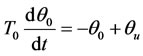
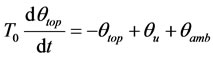
This is a classical model for predicting TOT of power transformer. TOT rise over ambient temperature is defined in a differential equation as below [8]:
 (1)
(1)
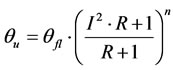
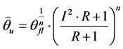
where q0 is top-oil temperature rise over ambient temperature, T0 is time constant at nominal load and qu is ultimate top-oil temperature rise due to load and is expressed as the following equation:
 (2)
(2)
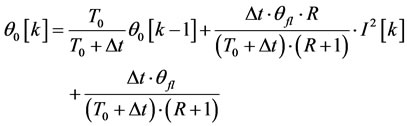
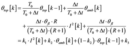
where qfl is top-oil temperature rise over ambient temperature at nominal load, R is the ratio of load loss at rated load to no-load loss, I is ratio of the specified load to rated load and n is oil cooling state exponent. Assuming n ≈ 1, applying Euler discretion rule and after simplifying, TOT rise over ambient temperature is given in below equation:
 (3)
(3)
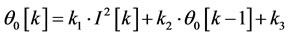
And by substituting coefficients k1, k2 and k3:
 (4)
(4)
This simplified model does not take dynamic variation of ambient temperature on TOT into account and in addition model accuracy is not acceptable.
2.2. Nonlinear Top-Oil Model
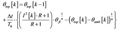
Nonlinear Top-Oil Model proposed in [9,10] explains dynamic variation in ambient temperature and is defined as below equation:
 (5)
(5)
In fact, this model is the correlated form of the model proposed in IEEE. To use Euler discretion method and n ≈ 1 we have:
 (6)
(6)
2.3. Swift Model
Swift model proposed in [11] is the change in exponential coefficient of oil in nonlinear model:
 (7)
(7)
 (8)
(8)
After discretion of Equation (7):
 (9)
(9)
Because of the form of nonlinearity in Equation (9), qtop[k] appears implicitly on both sides of the equation which makes training much difficult [7]. None of these models perform adequately when using parameters achieved from test report. However, all of these models perform adequately when their parameters are selected to optimally fit measured data [7]. When exponential coefficient of oil is one, it means that pumps and fans are working at rated condition; in this situation swift model is equal to the nonlinear top-oil model. Since fans and pumps are ON during the experiment, both of the models would have the same discrete model. The performance of first model is not acceptable due to excluding variations of environmental temperature. It was mentioned that Swift model and nonlinear model are equal so Equation (6) is used as final model and coefficients will be obtained through experimental data.
3. Optimization Algorithms
In this paper, three methods are used so to obtain the coefficients of Equation (6). Our target is comparing the results of proposed methods as well as the improvements in the limiting of variations in the coefficients.
3.1. Multiple-Linear Regression (M-L R)
The method used for multiple-regression is an extension of which used for single regression. For a model with three independent variables and in scalar form, output is rewritten as:
 (10)
(10)
where:
x1: Load value;
x2: Ambient temperature;
x3: TOT(k − 1);
 : Predicted TOT(k);
y: Actual TOT(k);
e: Error of prediction;
k1, k2, k3: Coefficient to be determined.
In vector form, Equation (10) can be written
 (11)
(11)
where Y is a 3 ´ 1 vector, X is a 3 ´ k matrix of sampled variables, K is a k ´ 1 vector of the coefficients, K0 is a 3 ´ k vector of constant scalar values and E is a 3 ´ 1 vector of random errors. In order to determine coefficients, those values are selected when the squared error between the actual TOT and the predicted TOT is minimized. This criterion can be expressed as:
 (12)
(12)
The least-squares estimate coefficients as below:
 (13)
(13)
In order to find the coefficients that minimize the squared error, Equation (12) can be solved with optimization algorithms such as GA and PSO.
3.2. Genetic Algorithm
The genetic algorithm (GA) is an optimization and search technique based on the principles of genetics and natural selection. GA allows a population composed of many individuals to evolve under specified selection rules in a state that maximizes or minimizes the fitness function [12,13]. N data-sets are selected in specific domain. Data-sets are substituted in fitness function and they are scaled and then all of them are scored. Children of the next generation can be produced from parents in the current generation according to the following methods:
• Selection of parents (Elite).
• Cross over.
• Mutation.
The procedure will continue until one of the stopping criteria is met. Some of the stopping criteria are discussed in below:
• A solution is found that satisfies minimum criteria.
• Allocated budget (computation time) reached.
• Fixed number of generations reached.
• Successive iterations no longer produce better results.
In this paper, fitness function is defined as the follow equation:
 (14)
(14)
where, N is the number of data used for finding of the coefficients.
3.3. Particle Swarm Optimization (PSO) Algorithm
In the PSO algorithm each individual is called a particle, and it is subjected to a movement in a multidimensional space that represents the belief space. Particles have memory and thus retain part of their previous state. There is no restriction for particles to share the same point in belief space, but their individuality is preserved in any case. Each particle’s movement is the composition of an initial random velocity and two randomly weighted influences [14]:
• Individuality: the tendency to return to the particle’s best previous position.
• Sociality: the tendency to move towards the neighborhood’s best previous position.
The velocity of each particle in the swarm is updated by using the following equation:
 (15)
(15)
wherevi(t): the velocity of particle i at time t;
xi(t): the position of particle i at time t;
w, c1, c2: user-supplied coefficients;
r1, r2: random values regenerated for each velocity update;
 : the individual best candidate solution for particle i at time t;
g(t): the best swarm’s global candidate solution at time t.
The objective function is the same function in GA method.
4. Coefficients Calculation
In order to increase precise of the model, all experimental data is converted to per unit values. Nominal values are:
P = 5 (MVA)
TOT = 55 (˚C)
qambient = 35 (˚C)
Using per unit values is an essential fact which is sometimes forgotten. For example, if values are not converted to per unit, load will have greater value comparing to temperature. In this case, changes of load would be greater comparing to thermal changes which results inappropriate effect of temperature on the model. In addition, using per unit values would decrease the range of coefficients changes. Coefficients obtained from PSO, GA and linear regression in five time intervals are given in Table 1. k1 is the most important coefficient since it shows the effect of load on temperature. The range of coefficients changes is limited in an appropriate model. In order to obtain global coefficients, all data is used. Results are given in Table 2. In order to show the performance of the model as well as its precision and accuracy in TOT modeling, limited data numbers are used to predict TOT in all ranges and then results are compared with the original values. Estimated and actual values of TOT are compared in Figure 1. Table 3 shows error of predicted TOT.
The load range used for testing the model is wide and results show that PSO has a good performance. Mean relative error is not the only parameter which evaluates

Table 1. Coefficients of the model.
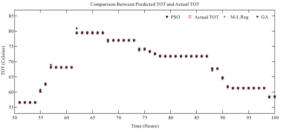
Figure 1. Comparison between predicted TOT and actual TOT.
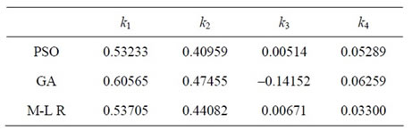
Table 2. Obtained coefficients from all of data.
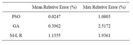
Table 3. Error of predicted TOT.
performance of the model. High value of error in prediction causes a mistake in choosing the load of transformer and in many cases this mistake raises the oil temperature dramatically to a high degree and causes harmful effects. Predicting TOT higher than its real value makes the operator to reduce loading which is not harmful for transformer. However, if the predicted value of TOT is fewer than its original value, operator would increase load and it may cause actual TOT to become higher than its permitted value while the predicted TOT is in permitted range. Repeating this action would accelerate the aging process.
5. Model Assessment
5.1. Adequacy
Adequacy measure whether the model has an appropriate structure to capture the features of the process being modeled. Residual versus fitted value diagrams are used to examine the adequacy of the model [7]. A typical diagram of residual versus fitted value is shown in Figure 2.
Figure 2(a) shows example of a good adequacy but Figure 2(b) means nonlinearity in the model and there will be the need for having other variables. On the other hand, some variables have not been considered in the model. R(i) verses TOT(i) is illustrated in Figure 3. It is obvious that the model is adequate and does not need additional variables.

Figure 2. Typical residual vs fitted value.
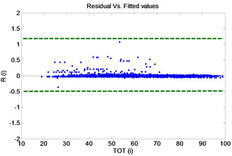
Figure 3. Achieved residual vs fitted value.
5.2. Consistency
Consistency is a quantitative measuring of the model’s ability and solution method to produce the same model parameter when training to use similar data. A standard deviation (STD) of parameters is used to examine consistency. For this purpose, “p” independent but similar data-sets are used for calculating coefficients. The STD of the model coefficients is calculated with Equation (16):
 (16)
(16)
Table 4 shows STD for each coefficient. It is clear that standard deviations of coefficients obtained from optimization algorithms have smaller values.
5.3. Accuracy
The typical metric used for assessing model accuracy is R2. The R2 metrics measure how well the predicted values (i.e., TOTpredicted) capture the variation of measured values (i.e., TOTactual):
 (17)
(17)
where, SSR is the sum of residuals square and measures the variation of predicted values. The variable SST is the total variation of measured values. The R2 value close to 1 indicates that values of the model closely match those which are measured. Table 5 shows the values of R2 for three models.
6. Conclusion
In this paper, three models are introduced for predicting
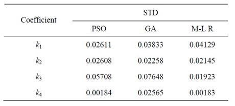
Table 4. STD of achieved coefficients.
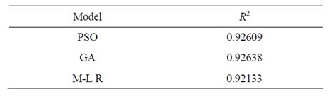
Table 5. Obtained value of R2 from three models
top oil temperature (TOT) in power transformers. GA and PSO are used so to define coefficients of models through experimental data. PSO algorithm leads to the best performance with considering the achieved results. The main success is limited ranges of coefficients especially for k1 (effect of load on temperature). In addition, mean relative error becomes near zero. In the paper was shown that nonlinear model is a good model itself, but obtaining the coefficients with traditional method cause inappropriate performances of the nonlinear model. New optimization algorithms improve performances of this model related to multi-linear regression. Additionally, it was depicted that using optimization algorithms improves the model adequacy, consistency as well as accuracy.
REFERENCES
- M. A. Taghikhani and A. Gholami, “Temperature Distribution in ONAN Power Transformer Windings with Finite Element Method,” European Transactions on Electrical Power, Vol. 19, No. 5, 2009, pp. 718-730. doi:10.1002/etep.251
- Z. Radakovic, “Numerical Determination of Characteristic Temperatures in Directly Loaded Power Oil Transformer,” European Transactions on Electrical Power, Vol. 13, No. 1, 2003, pp. 47-54. doi:10.1002/etep.4450130107
- L. Jauregui-Rivera, X. L. Mao and D. J. Tylavsky, “Improving Reliability Assessment of Transformer Thermal Top-Oil Model Parameters Estimated from Measured Data,” IEEE Transactions on Power Delivery, Vol. 24, No. 1, 2009, pp. 169-176. doi:10.1109/TPWRD.2008.2005686
- K. P. Jouni, K. Nousiainen and P. Verho, “Studies to Utilize Loading Guides and Ann for Oil-Immersed Distribution Transformer Condition Monitoring,” IEEE Transactions on Power Delivery, Vol. 22, No. 1, 2007, pp. 201- 207. doi:10.1109/TPWRD.2006.877075
- Q. He, J. Si and D. J. Tylavsky, “Prediction of Top-Oil Temperature for Transformers Using Neural Networks,” IEEE Transactions on Power Delivery, Vol. 15, No. 4, 2000, pp. 1205-1211. doi:10.1109/61.891504
- H. Nguyen, G. W. Baxter and L. Reznik, “Soft Computing Techniques to Model the Top-Oil Temperature of Power Transformers,” International Conference on Intelligent Systems Applications to Power Systems (ISAP), Taiwan, 5-8 November 2007, pp. 1-6. doi:10.1109/ISAP.2007.4441618
- L. Jauregui-Rivera and D. J. Tylavsky, “Acceptability of Four Transformer Top-Oil Thermal Models—Part I: Defining Metrics,” IEEE Transactions on Power Delivery, Vol. 23, No. 2, 2008, pp. 860-865. doi:10.1109/TPWRD.2007.905555
- IEEE Standard, C57.91-1995, “IEEE Guide for Loading Mineral Oil Immersed Transformer,” 1996.
- B. C. Lesieutre, W. H. Hagman and J. L. Jr. Kirtley, “An Improved Transformer Top Oil Temperature Model for Use in an On-Line Monitoring and Diagnostic System,” IEEE Transactions on Power Delivery, Vol. 12, No. 1, 1997, pp. 249-256. doi:10.1109/61.568247
- D. J. Tylavsky, X. L. Mao and G. A. McCulla, “Transformer Thermal Modeling: Improving Reliability Using Data Quality Control,” IEEE Transactions on Power Delivery, Vol. 21, No. 3, 2006, pp. 1357-1366. doi:10.1109/TPWRD.2005.864039
- G. Swift, T. Molinski, W. Lehn and, R. Bray, “A Fundamental Approach to Transformer Thermal Modeling— Part I: Theory and Equivalent Circuit,” IEEE Transactions on Power Delivery, Vol. 16, No. 2, 2001, pp. 171- 175. doi:10.1109/61.915478
- R. L. Haupt and S. E. Haupt, “Practical Genetic Algorithms,” 2nd Edition, John Wiley & Sons Inc. Publication, Hoboken, 2004.
- V. Galdi, L. Ippolito, A. Piccolo and A. Vaccaro, “Parameter Identification of Power Transformers Thermal Model via Genetic Algorithms,” Electric Power Systems Research, Vol. 60, No. 2, 2001, pp. 107-113. doi:10.1016/S0378-7796(01)00173-0
- W. H. Tang, S. He, E. Prempain, Q. H. Wu and J. Fitch, “A Particle Swarm Optimizer with Passive Congregation Approach to Thermal Modeling for Power Transformers,” The 2005 IEEE Congress on Evolutionary Computation, Vol. 3, 2005, pp. 2745-2751.