Atmospheric and Climate Sciences
Vol.3 No.4(2013), Article ID:36697,10 pages DOI:10.4236/acs.2013.34048
Model-Measurement Comparison of Ammonia Bi-Directional Air-Surface Exchange Fluxes over Agricultural Fields
1Air Quality Research Division, Science and Technology Branch, Environment Canada, Toronto, Canada
2Stratford, Canada
Email: *leiming.zhang@ec.gc.ca
Copyright © 2013 Zhuanshi He et al. This is an open access article distributed under the Creative Commons Attribution License, which permits unrestricted use, distribution, and reproduction in any medium, provided the original work is properly cited.
Received July 17, 2013; revised August 16, 2013; accepted August 23, 2013
Keywords: Air-Quality Model; Dry Deposition; Soil Emission; Model Evaluation
ABSTRACT
Modeled and measured bi-directional fluxes (BDFs) of ammonia (NH3) were compared over fertilized soybean and corn canopies for three intensive sampling periods: the first, during the summer of 2002 in Warsaw, North Carolina (NC), USA; and the second and third during the summer of 2007 in Lillington, NC. For the first and the third experimental periods, the BDF model produced reasonable diurnal flux patterns. The model also produced correct flux directions (emission and dry deposition) and magnitudes under dry and wet canopy conditions and during day and nighttime for these two periods. However, the model fails to produce the observed very high upward fluxes from the second sampling period due to the fertilization application (and thus being much higher soil emission potentials in the field than the default model values), although this can be improved by adjusting model input of soil emission potentials. Model-measurement comparison results suggest that the model is likely capable for improving long-term or regional scale ammonia predictions if implemented in chemical transport models replace the traditional dry deposition models, although modifications are needed when applying to specific situations.
1. Introduction
Ammonia (NH3) plays important roles in atmospheric chemical processes and biogeochemical cycles [1-3]. NH3 is a major contributor to secondary inorganic aerosol compounds [4,5] which affect air quality and have direct and indirect impacts on climate [6]. NH3 and ammonium ( ) represent important nutrients to the biosphere in some areas, and their deposition can fertilize nitrogen-limited ecosystems. NH3 and
  can also have detrimental effects such as eutrophication, soil acidification, and the loss of biodiversity in sensitive ecosystems [7-10].
The primary sources of NH3 are animal waste, ammonification of humus followed by emission from soils, losses of NH3-based fertilizers from soils, and industrial emissions [11]. The majority of these emissions come primarily from biological processes, as well as from byproducts of agricultural and waste production and processing of both human and animal waste [12-14]. A significant fraction of NH3 emitted from major sources can be dry deposited to local areas downwind of the source [15,16]. However, measurements have shown that vegetation can be a source or a sink of atmospheric NH3 [17- 19], and biological processes in soils enriched by reduced nitrogen (NHx) can lead to emissions of NH3 [20].
Atmospheric chemical transport models (CTMs) are useful tools to assess pollutant fate and impact on ecosystems and to provide source-receptor relationships which can be used for making emission control policies. Anthropogenic NH3 emission sources are mostly included in the input files of CTMs, but the biogenic emissions might not be treated properly due to the coupling process between dry deposition and emission. One approach proposed in the literature is to use a bi-directional flux (BDF) scheme to replace the dry deposition only scheme [21]. In comparison to the rather simplified dry deposition scheme (non-BDF) currently used in CTMs, the BDF scheme accounts for not only deposition but also emission over certain land-use types. Depending on the ambient mixing ratio, the BDF scheme could 1) lead to larger fluxes from the surface to the atmosphere [5, 17,18,22-25]; and 2) improve the performance of NH3 prediction, leading to a better understanding of the ecosystem nitrogen budget.
Although the improvements to the parameterization methods involving vegetation-atmosphere bi-directional NH3 exchange depending on the mixing ratios of NH3 near the ground surface were reported recently in Europe and North America [26-30], performance testing of the bi-directional exchange scheme and measurements is still under development in North America [31-34]. A comprehensive review of the various recently-developed models for the air-surface exchange of NH3, as well as an in-depth examination of the theory and measurements from which the models are developed and tested, can be found in Flechard et al. (2013) [35]. In this study, we aim to evaluate the performance of the bi-directional dry deposition scheme of Zhang et al. (2010) [30] using measured bi-directional fluxes of NH3 over fertilized soybean during the summer of 2002 in Warsaw, North Carolina (NC), USA, and over a fertilized corn canopy during the summer of 2007 in Lillington, NC. Another purpose of the study is to compare the air-surface exchange processes of NH3 under various wetness conditions.
2. Methodology
2.1. Measurements
Measurements were carried out at two sites (Warsaw and Lillington, NC, USA) during three intensive sampling periods. One sampling period was in Warsaw, over a fertilized soybean field, and the other two sampling periods were in Lillington, over a fertilized corn canopy. These three periods capture the full range of flux conditions from deposition to strong emission. Measurements conducted over these two plants, and over a wide range of soil, vegetation, and atmospheric conditions, should help in understanding NH3 flux characteristics over different land-use types. Several meteorological variables were also sampled at the same time as the flux measurements.
2.1.1. Warsaw (Site 1)
The first site (hereafter referred to as Site 1), was a 90 ha fertilized soybean [Glycine max (L.) Merr.] field in Warsaw, North Carolina. The bi-directional NH3 fluxes were measured from 06/17/02 to 08/22/02 using the modified Bowen-ratio method. These data represent measurements of a soybean crop in the middle of its growing season and exposed to relatively high atmospheric NH3 concentrations due to local fertilization and NH3 emissions from nearby animal production facilities. The reader is referred to Walker et al. (2006) [19] for a more detailed description of the site and measurements.
2.1.2. Lillington (Site 2)
The second site was a 200 ha fertilized corn (Zea mays, Pioneer varieties 31G66 and 31P41) field in Lillington, North Carolina. The above-canopy NH3 fluxes presented here cover two periods: from 06/21/07 to 06/29/07 (hereafter referred to as Lillington-A or Site 2a) and from 07/ 06/07 to 07/31/07 (hereafter referred to as Lillington-B, Site 2b), using the modified Bowen-ratio method. These data represent measurements of a corn canopy in the middle of its growing season and high in NH3 due to fertilization with a urease inhibitor. An extensive description of these measurements can be found in Walker et al. (2013) [34].
2.1.3. Data Grouping
To evaluate the bi-directional model and compare with measurements, the original measured datasets were prescreened with the condition that both the measured NH3 concentrations and bi-directional fluxes must be available. Data were then grouped into different categories using criteria defined in Zhang et al. (2002) [36] as listed in Table 1. The purpose of grouping the data this way is to investigate the air-surface exchange processes under different wetness conditions. Note that the model to be evaluated here also treats the non-stomatal uptake differently for dry and wet canopies.
The first group includes the entire dataset used in the analysis (G1), the second group is for a dry canopy with low relative humidity (RH) (G2), the third group is for dry canopy but with high RH (G3), and the fourth (G4) and fifth (G5) groups are for wet conditions caused by dew and rain, respectively. N is the number of halfhourly observations under each category. The data were also grouped as G2 and non-G2 (=G3 + G4 + G5) and separated into daytime (07:30-19:00) and nighttime (19:30-07:00) datasets for further comparison. During data pre-screening, observations grouped into G2 at a specific time were re-checked to determine if rain occurred at any point during the previous four records. If so, then the data were re-grouped into both non-G2 and G5 (Wet-Rain) groups. The total number of post-processed observations for Warsaw (Site 1), Lillington-A (Site 2a), and Lillington-B (Site 2b) were 1383, 307, and 546, respectively. All fluxes discussed hereafter refer to the post-screened data of the bi-directional fluxes of NH3.
2.2. Bi-Directional Flux Modeling
The bi-directional flux exchange over the leaf stomata and over soil in our BDF model is very similar to the two-layer model of Nemitz et al. (2001) [25], and is similar in concept to the existing bi-directional air-sur-

Table 1. Data grouping criteria and the numbers of data samples (N) for the three campaigns (S1, S2a and S2b). G3 group represents dry condition but with high relative humidity (RH). Numbers of samples in bracket are for daytime (07:30-19:00) and nighttime (19:30-07:00), respectively.
face exchange models developed for NH3 [16,21,26,34, 37-40]. The major differences between our BDF and other models include 1) different positioning of Rb (the quasi-laminar sublayer resistance) in the resistance analogy, 2) different parameterizations for resistance components, and 3) parameter values chosen for emission potentials over various land-use categories (LUCs).
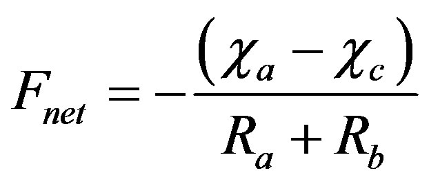
The net flux of NH3 (Fnet) is calculated according to the equation:
 (1)
(1)
where ca is the ambient concentration at the reference height; cc is the ambient concentration at the canopy top; Ra is the aerodynamic resistance, a function of micrometeorological conditions only; and Rb is a function of the friction velocity (u*) and the molecular diffusivity of each chemical species. To reduce the uncertainty in the numerical simulation, the measured u* was used, when available, during the calculations. The direction of the flux is related to the difference between ca and cc, where a positive flux implies emission and a negative flux implies deposition. The reader is referred to Zhang et al. (2003 and 2010) [30,41] for the detailed parameterization of the model.
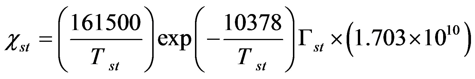
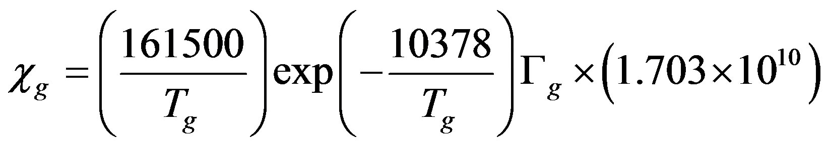
Compared with the non-BDF model, the BDF model requires the compensation points (at which flux change directions) over the stomata (χst) and over the soil (χg), which are given in μg∙m−3 by [25,42]:
 (2a)
(2a)
 (2b)
(2b)
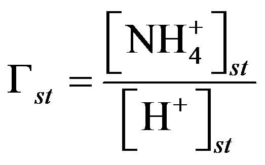
where Tst is the temperature of the leaf stomata (K), Гst is the stomatal emission potential (also known as the apoplastic ratio) at 1 atmosphere, Tg is the temperature of the ground surface (K), and Гg is the soil emission potential. The emission potentials are defined as [38,42]:
 (3a)
(3a)
 (3b)
(3b)
where  and
and  are the concentrations of
  (mol∙L−1) in the apoplastic fluid and in the soil/surface litter, respectively; [H+]st and [H+]g are the concentrations of H+ in the apoplastic fluid and soil/surface litter, respectively. Empirically derived values for Гst and Гg were defined for each LUC, with a total of twenty-six LUCs in the BDF model (see [30] for a detailed review of these values over different LUCs). Measured Гst and Гg (calculated from measured
  and [H+] in both the leaf apoplast and soil) were used in the sensitivity tests (Section 3.3). In this study, LUCs 15 (crops) and 18 (maize) were the two LUCs assigned for Warsaw (Site 1) and Lillington-A, B (Sites 2a, b), respectively.
3. Results
3.1. Summary of Measured Concentrations and Bi-Directional Fluxes of Ammonia
A summary of the half-hourly concentrations and bidirectional fluxes of NH3 measured during the three sampling periods is provided in Table 2. The mean, minimum, and maximum values are shown for all five groups for both the daytime and the nighttime. A positive mean flux implies that emission was dominant, while a negative mean flux indicates that deposition was dominant during the given conditions.
3.1.1. Warsaw, Site 1, 06/18/02 to 08/22/02
NH3 concentrations over the soybean field ranged from 0.01 to 35.3 μg∙m −3, with mean and median values of 9.7 ± 6 and 9.0 μg∙m−3 (N = 1383), respectively. These values from the post-screened dataset are comparable to those of the original dataset reported by Walker et al.
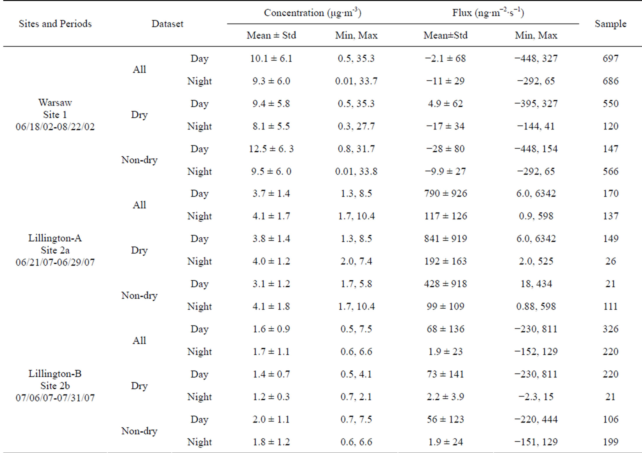
Table 2. Summary of measured ammonia concentrations and fluxes.
(2006) [19] (0.01 to 43.9, 9.4, and 8.6 μg∙m−3, N = 1599). The differences in average concentrations were in the range of 10% - 30% between day and night and between dry and non-dry conditions (Table 2). For the whole dataset (G1), the average flux was −6.6 ± 52 ng∙m−2∙s−1, and ranged from −448 to 326 ng∙m−2∙s−1. Both emission and deposition fluxes were observed during the day or night and under dry or non-dry conditions. A net emission of NH3 (4.9 ± 62 ng∙m−2∙s−1) was observed under dry daytime condition while net deposition was observed under other conditions.
3.1.2. Lillington-A, Site 2a, 06/21/07 to 06/29/07
NH3 concentrations over the corn field in June ranged from 1.3 to 10.4 μg∙m−3, with mean and median values of 3.9 ± 1.5 and 3.6 μg∙m−3 (N = 307), respectively. The differences in average concentrations were around 5% - 30% between day and night and between dry and non-dry conditions. The measured flux ranged from 0.9 to 6342 ng∙m−2∙s−1, with mean and median values of 489 ± 770 and 243 ng∙m−2∙s−1, respectively. This means that only emission fluxes (no dry deposition fluxes) were observed during this period. The measured emission fluxes in the daytime were four-to-six times larger than those in the nighttime. Apparently, the fertilization of the corn field two weeks prior to the measurements was still contributing to the NH3, leading to strong emissions during both the daytime and nighttime [34].
3.1.3. Lillington-B, Site 2b, 07/06/07 to 07/31/07
NH3 concentrations over the corn field during the month of July ranged from 0.5 to 7.5 μg∙m−3, with mean and median values of 1.6 ± 1 and 1.3 μg∙m−3 (N = 307), respectively. No significant differences (mostly <10%) were found in the average concentrations under different conditions (Table 2). The measured flux ranged from −230 to 811 ng∙m−2∙s−1, with mean and median values of 41 ± 111 and 6 ng∙m−2∙s−1, respectively. Similar to Lillington-A (Site 2a), small values, close in range, for the NH3 concentrations were obtained for this sampling period at the same site. However, the mean measured positive flux in the daytime was 30 - 34 times the flux in the nighttime, likely due to the higher friction velocity during the day and the smaller emission potential in the soil during this sampling period, as the effect of the fertilization is diminished. One can conclude that emissions were still the dominant bi-directional air-surface exchange
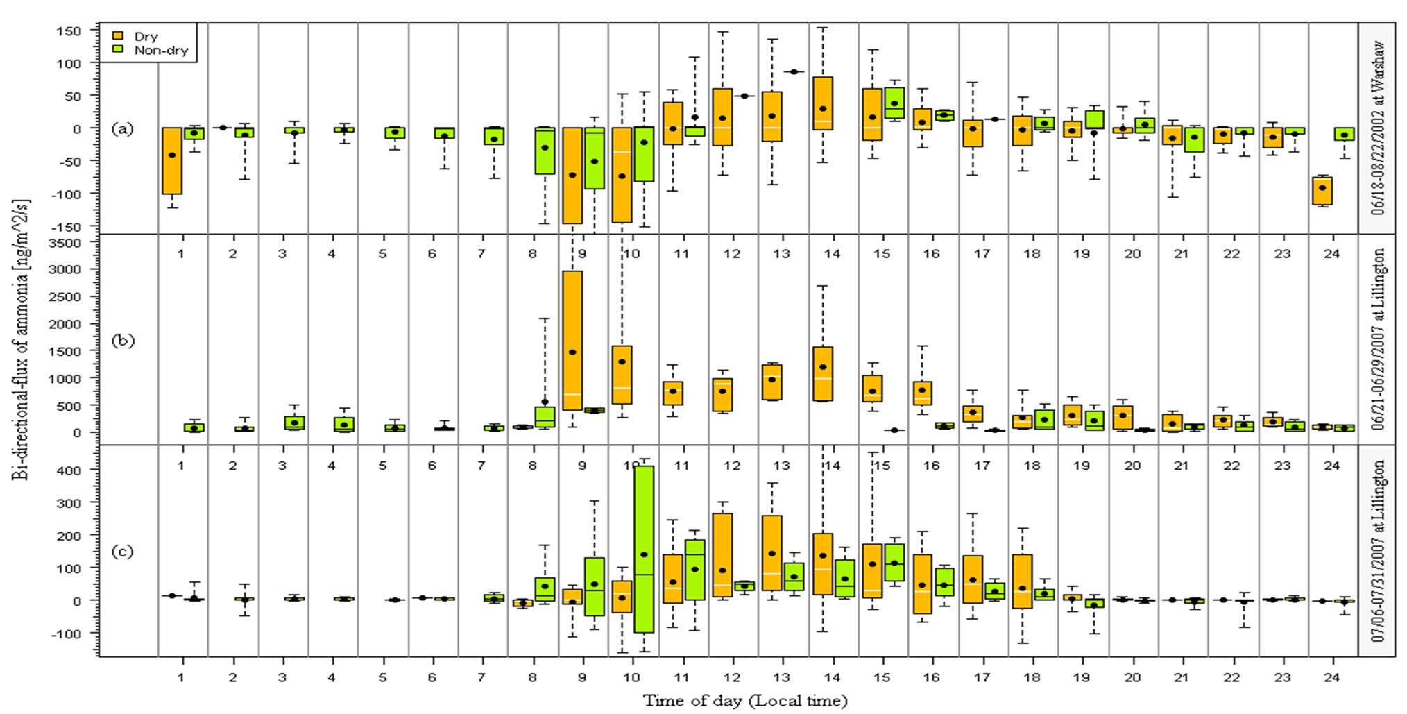
Figure 1. Diurnal variations of measured bi-directional fluxes of ammonia for dry and non-dry datasets. The values presented on box-and-whisker plots are 5, 16.5, 50, 83.5 and 95 percentile (the central 67% and 95% data are shown), and the black dots represent the mean values.
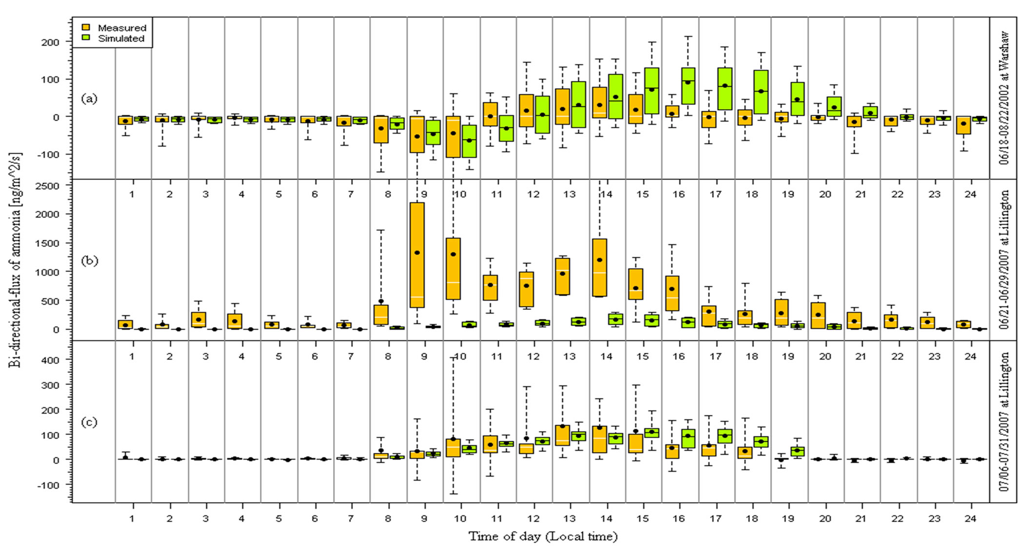
Figure 2. Diurnal variation of measured and modeled bi-directional fluxes of NH3 using default parameters of BDF model. The box-and-whisker plots are the same as in Figure 1.
pathway during the sampling period.
3.1.4. Diurnal Variations for Dry and Non-Dry Datasets
The diurnal patterns of the measured fluxes for G2 and non-G2 conditions are shown in Figure 1, in which the original half-hourly data were averaged into hourly data. At Site 1 which had the lowest soil N among the three campaigns, fluxes were mostly downward during the nighttime and early morning and mostly upward from mid-morning to late afternoon under both dry and nondry conditions. At Site 2a which had the highest soil N content due to fertilization, upward fluxes were observed during most of the day and nighttime, and the fluxes were much higher during the day than the night and were also higher under dry than wet conditions. At Site 2b which had higher soil N than at Site 1 but lower N than at Site 2a, both upward and downward fluxes were observed during nighttime although daytime fluxes were mostly upward. With solar radiation warming the soil and leaf surfaces during the daytime, evaporation produces an emission from the soil and leaves, resulting in a higher emission flux. Theoretically, under non-dry conditions, water in the soil and dewdrops on the leaf surfaces can absorb NH3, thereby leading to lower emissions and therefore lower fluxes. Thus, wetness generally increases downward fluxes and decreases upward flux. However, very high pH in the surface droplets will reduce the ability of the canopy to absorb NH3 under wet conditions and actually lead to higher emission fluxes during wet conditions. This phenomenon was actually observed during the Lillington corn experiment. Besides, the evaporation of morning dew can also increase upward fluxes. Apparently, the directions of fluxes and diurnal patterns depended on the meteorological and canopy conditions as well as the soil N content.
3.2. Model-Measurement Comparison
3.2.1. Diurnal Variation
Figure 2 shows the model-measurement comparisons of the diurnal variations of hourly-averaged fluxes for the three campaigns. Modeling simulations using the default parameters for the BDF model (LAI, Гst, and Гg, etc.)
were conducted corresponding to the post-screened data. All 30-min data were averaged hourly, for both the measurements and the modeling estimates.
As expected, the fluxes during the nights were lower than in the daytime, due to increased emissions from the soil caused by solar radiation and greater turbulent mixing during the day. In general, the mean flux gradually increased in the morning after 08:00 and reached a peak approximately five or six hours later. The highest flux was commonly observed between 12:00 and 16:00. The diurnal variation profile of the measured flux peaked at 14:00 and 13:00 at Site 1 (Figure 1(a)) and Site 2b (Figure 1(c)), respectively. The top three mean fluxes of NH3 at Site 2a were observed at 09:00, 10:00, and 14:00. The first two peaks were mainly caused by the very large fluxes observed during the daytime on 06/22/07 (DOY 173), 06/24/07 (DOY 175), and 06/26/07 (DOY 177), which are most likely a result of a combination of a rainfall and then soil warming which caused a reaction in the fertilizer in the soil [34].
The model captured the observed diurnal trends well at Site 1 and Site 2b. The resulting modeled and measured fluxes were found to be in good agreement during these two campaigns. The modeled and measured fluxes were −1.9 ± 28 and −6.6 ± 52 ng∙m−2∙s−1 at Site 1, and 41 ± 50 and 41 ± 110 ng∙m−2∙s−1 at Site 2b, respectively. However, the modeled fluxes were much smaller than the observed fluxes between 08:00 and 20:00 at Site 2a due to the very high soil  concentration (Figure 1(b)) (see Section 3.3 for more discussion) and corresponding soil emission potential (Gg).
3.2.2. Comparisons under Different Meteorological Conditions
To evaluate the performance of the BDF model under different meteorological conditions, the statistics of the measured and modeled fluxes for groups G2-G5 in the daytime and nighttime for Site 1 and Site 2b are shown in Figure 3. The model performed reasonably well compared to the measurements. For example, the model produced correct flux directions and magnitudes at both Site 1 and Site 2b under the majority of conditions during both day and night periods. There were a few cases when the model differed significantly from the measurements. These include day and nighttime dry conditions at Site 1 when the model produced too high emission fluxes than the measurements, daytime dew condition at Site 2b when the model did not produce as high emission fluxes as measurements, and daytime rain condition at Site 1 and nighttime rain condition at Site 2b when the model produced more deposition than emission fluxes while the measurements showed the other way around. For Site 1, slightly decreasing the soil emission potential used in the model should improve the model’s overall performance at this site. For Site 2b, the large range of measured flux values under daytime dew conditions would not be achieved by simply modifying one or two model default parameters because the observed phenomena were caused by a combination of various meteorological and chemical conditions that were not all considered in the BDF model. Overall, the BDF modeled fluxes were significant improvements compared to the non-BDF model results which would only have downward fluxes.
3.3. Sensitivity Tests
The initial results from the BDF model, such as the mean fluxes and trends in the diurnal variation, agree well with the measurements for Sites 1 and 2b using the default model parameters as discussed above. However, due to the much high soil N content at Site 2a, the model fails to produce the high emission fluxes during the daytime. The measured Гg (=[NH4]/[H+]) at this site ranged from 180 to 2,523,893, with mean and median values of 120,482 ± 315,700 and 15,356, respectively. In comparison, the model default value of Гg is 5000. Thus, model sensitivity tests using larger Гg values were conducted (Figure 4). An addition test was also included by changing the surface roughness length which was expected to change resistance terms and then modeled fluxes.

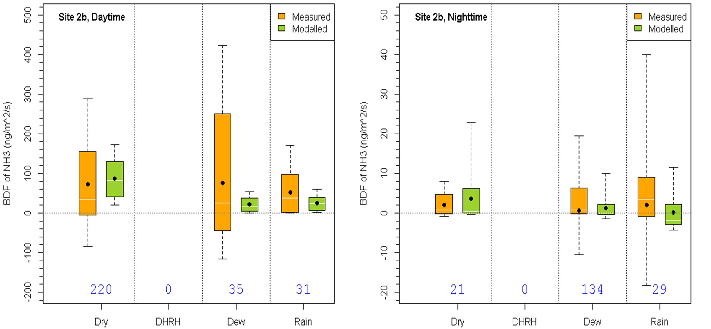
Figure 3. Comparison of measured and modeled fluxes under various conditions specified in Table 1 for Sites 1 (top row) and 2b (bottom row) during dayand nighttime. The box-and-whisker plots are the same as in Figure 1.
When Гg was increased to 50,000 (Test 1), which was 10 times larger than the model default value but was less than half of the measured average value, modeled upward fluxes increased substantially and matched the measured values during afternoon and evening time, although still lower than measured values during early morning and late nighttime. When Гg was further increased to 65,000 (Test 2), modeled upward flux matched measured values from mid-morning to noon time, higher in the afternoon, still lower in the early morning. As mentioned earlier, the high fluxes observed at 09:00-10:00 were caused by the very large fluxes from three days (DOY 173, 175 and 177). Using a Гg smaller than the measured median value cannot generate such high fluxes.
Using the same Гg as in Test 2 but using a larger roughness length (Test 3), modeled fluxes also increased slightly during daytime. The average modeled and measured fluxes were 447 ± 527 and 489 ± 771 ng∙m−2∙s−1, respectively, from sensitivity Test 3. The above sensitivity tests suggest that Гg is the most important model parameter for agricultural landscapes, although other parameters also play a role in the model fluxes. The model can capture the large diurnal upward fluxes if more realistic soil emission potential parameter is available.
4. Conclusions
A bi-directional flux of the atmospheric NH3 model was
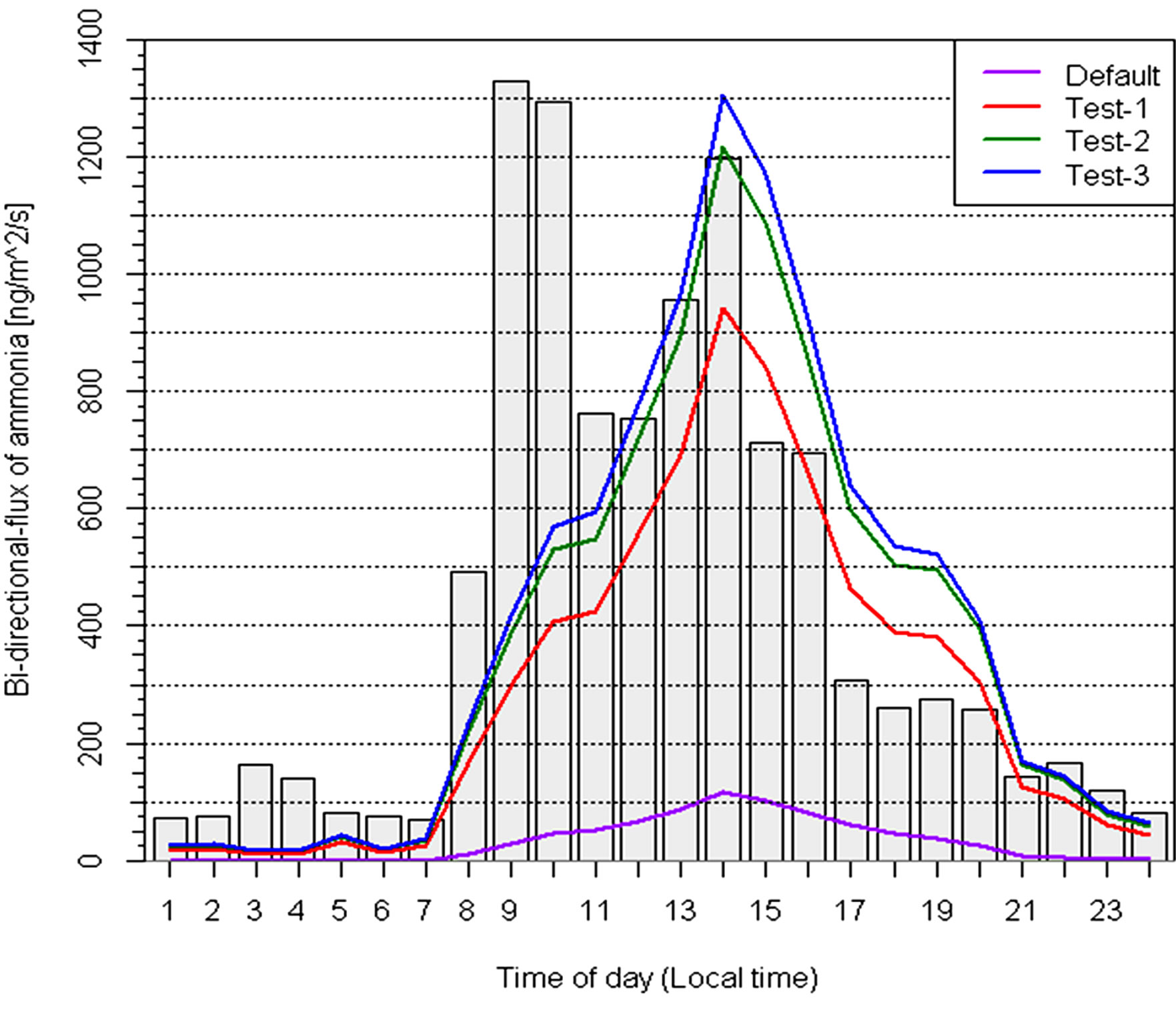
Figure 4. Sensitivity test for Site 2a. Grey bars and purple dashed line represent the observation and default model run, respectively.
evaluated based on three sets of measurements over two different agricultural land-use categories during the summer. On conditions of no fresh fertilization, the model captures the diurnal pattern of observed fluxes, an obvious improvement over the original NH3 dry deposition model. If fertilizer was applied, the model would fails to capture the very large upward flux with default model parameters. With adjusted model parameter of soil emission, a better agreement between model and measurements can be achieved. However, when applying the model in regional scale chemical transport models, care should be given to the choice of soil emission parameters. This is because anthropogenic emission is most likely included in a separate emission input file. The bi-directional flux model should not introduce additional high emission flux if that is already considered in emission inputs. This will not be a concern when applying the model to specific sites.
While soil emission is more important than leaf stomata emission over agricultural landscapes, it is the other way around over natural forests. Thus, data should be collected over forest areas and used for evaluating the model. The model should also be evaluated at regional scales when implemented into chemical transport models. This work is underway for the Canadian air quality models [43].
5. Acknowledgements
We greatly appreciate John Walker of USEPA for providing the measurement data and critical comments on the paper.
REFERENCES
- A. S. Ansari and S. N. Pandis, “Response of Inorganic PM to Precursor Concentrations,” Environmental Science and Technology, Vol. 32, No. 18, 1998, pp. 2706-2714. http://dx.doi.org/10.1021/es971130j
- C. L. Blanchard and G. M. Hidy, “Effects of Changes in Sulfate, Ammonia, and Nitric Acid on Particulate Nitrate Concentrations in the Southeastern United States,” Journal of the Air and Waste Management Association, Vol. 53, No. 3, 2003, pp. 283-290. http://dx.doi.org/10.1080/10473289.2003.10466152
- D. V. Vayenas, S. Takahama, C. I. Davidson and S. N. Pandis, “Simulation of the Thermodynamics and Removal Processes in the Sulfate-Ammonia-Nitric Acid System during Winter: Implications for PM2.5 Control Strategies,” Journal of Geophysical Research D: Atmospheres, Vol. 110, No. D7, 2005, pp. 1-11. http://dx.doi.org/10.1029/2004JD005038
- B. J. Finlayson-Pitts and J. N. Pitts, “Chemistry of the Upper and Lower Atmosphere: Theory, Experiments, and Applications,” Academic Press, San Deigo, 1999.
- R. A. Ellis, J. G. Murphy, M. Z. Markovic, T. C. Vandenboer, P. A. Makar, J. Brook and C. Mihele, “The Influence of Gas-Particle Partitioning and Surface-Atmosphere Exchange on Ammonia during BAQS-Met,” Atmospheric Chemistry and Physics, Vol. 11, No. 1, 2011, pp. 133-145. http://dx.doi.org/10.5194/acp-11-133-2011
- IPCC, “Climate Change 2001, Working Group I: The Scientific Basis, Ch5,” 2013. http://www.ipcc.ch/ipccreports/tar/wg1/
- A. Fangmeier, A. Hadwiger-Fangmeier, L. Van der Eerden and H.-J. Jäger, “Effects of Atmospheric Ammonia on Vegetation: A Review,” Environmental Pollution, Vol. 86, No. 1, 1994. pp. 43-82. http://dx.doi.org/10.1016/0269-7491(94)90008-6
- R. Bobbink, M. Hornung and J. G. M. Roelofs, “The Effects of Air-Borne Nitrogen Pollutants on Species Diversity in Natural and Semi-Natural European Vegetation,” Journal of Ecology, Vol. 86, No. 5, 1998, pp. 717- 738. http://dx.doi.org/10.1046/j.1365-2745.1998.8650717.x
- J. N. Galloway, J. D. Aber, J. W. Erisman, S. P. Seitzinger, R. W. Howarth, E. B. Cowling and B. J. Cosby, “The Nitrogen Gas Cascade,” Bioscience, Vol. 53, 2003, pp. 341-356. http://dx.doi.org/10.1641/0006-3568(2003)053[0341:TNC]2.0.CO;2
- S. V. Krupa, “Effects of Atmospheric Ammonia (NH3) on Terrestrial Vegetation: A Review,” Environmental Pollution, Vol. 124, No. 2, 2003, pp. 179-221. http://dx.doi.org/10.1016/S0269-7491(02)00434-7
- J. H. Seinfeld and S. N. Pandis, “Atmospheric Chemistry and Physics, from Air Pollution to Climate Change,” 2nd Edition, Wiley-Interscience Publication, Hoboken, 2006.
- J. W. Erisman, A. Bleeker, A. Hensen and A. Vermeulen, “Agriculture Air Quality in Europe and the Future Perspectives,” Atmospheric Environment, Vol. 42, No. 14, 2008, pp. 3209-3217. http://dx.doi.org/10.1016/j.atmosenv.2007.04.004
- P. A. Makar, M. D. Moran, Q. Zheng, S. Cousineau, M. Sassi, A. Duhamel, M. Besner, D. Davignon, L.-P. Crevier and V. S. Bouchet, “Modelling the Impacts of Ammonia Emissions Reductions on North American Air Quality,” Atmospheric Chemistry and Physics, Vol. 9, No. 18, 2009, pp. 7183-7212. http://dx.doi.org/10.5194/acpd-9-5371-2009
- USEPA, “US Environmental Protection Agency: National Emission Inventory (NEI) Air Pollutant Emission Trends Data,” 2013. http://www.epa.gov/ttn/chief/trends/
- G. P. Draajers, W. P. Ivens, M. M. Bos and W. Bleuten, “The Contribution of Ammonia Emissions from Agriculture to the Deposition of Acidifying and Eutrophying Compounds onto Forests,” Environmental Pollution, Vol. 60, No. 1-2, 1989, pp. 55-66. http://dx.doi.org/10.1016/0269-7491(89)90220-0
- J. Walker, P. Spence, S. Kimbrough and W. Robarge, “Inferential Model Estimates of Ammonia Dry Deposition in the Vicinity of a Swine Production Facility,” Atmospheric Environment, Vol. 42, No. 14, 2008, pp. 3407- 3418. http://dx.doi.org/10.1016/j.atmosenv.2007.06.004
- G. D. Farquhar, P. M. Firth, R. Wetselaar and B. Weir, “On the Gaseous Exchange of Anunonia between Leaves and the Environment: Determination of the Ammonia Compensation Point,” Plant Physiology, Vol. 66, No. 4, 1980, pp. 710-714. http://dx.doi.org/10.1104/pp.66.4.710
- M. A. Sutton, J. K. Schjorring, G. P. Wyers, J. H. Duyzer, P. Ineson and D. S. Powlson, “Plant-Atmosphere Exchange of Ammonia,” Philosophical Transactions—Royal Society of London A, Vol. 351, No. 1696, 1995, pp. 261-278. http://dx.doi.org/10.1098/rsta.1995.0033
- J. T. Walker, W. P. Robarge, Y. Wu and T. P. Meyers, “Measurement of Bi-Directional Ammonia Fluxes over Soybean Using the Modified Bowen-Ratio Technique,” Agricultural and Forest Meteorology, Vol. 138, No. 1-4, 2006, pp. 54-68. http://dx.doi.org/10.1016/j.agrformet.2006.03.011
- A., Mosier, C. Kroeze, C. Nevison, O. Oenema, S. Seitzinger and O. Van Cleemput, “Closing the Global N2O Budget: Nitrous Oxide Emissions through the Agricultural Nitrogen Cycle: OECD/IPCC/IEA Phase II Development of IPCC Guidelines for National Greenhouse Gas Inventory Methodology,” Nutrient Cycling in Agroecosystems, Vol. 52, No. 2-3, 1998, pp. 225-248. http://dx.doi.org/10.1023/A:1009740530221
- M. A. Sutton, J. K. Burkhardt, D. Guerin, E. Nemitz and D. Fowler, “Development of Resistance Models to Describe Measurements of Bi-Directional Ammonia SurfaceAtmosphere Exchange,” Atmospheric Environment, Vol. 32, No. 3, 1998, pp. 473-480. http://dx.doi.org/10.1016/S1352-2310(97)00164-7
- M. A. Sutton, D. Fowler and J. B. Moncrieff, “The Exchange of Atmospheric Ammonia with Vegetated Surfaces. I: Unfertilized Vegetation,” Quarterly Journal— Royal Meteorological Society, Vol. 119, No. 513, 1993, pp. 1023-1045. http://dx.doi.org/10.1002/qj.49711951309
- M. A. Sutton, D. Fowler, J. B. Moncrieff and R. L. Storeton-West, “The Exchange of Atmospheric Ammonia with Vegetated Surfaces. II: Fertilized Vegetation,” Quarterly Journal—Royal Meteorological Society, Vol. 119, No. 513, 1993, pp. 1047-1070. http://dx.doi.org/10.1002/qj.49711951310
- W. A. H. Asman, M. A. Button and J. K. Schjørring, “Ammonia: Emission, Atmospheric Transport and Deposition,” New Phytologist, Vol. 139, No. 1, 1998, pp. 25-26. http://dx.doi.org/10.1021/es971130j
- E. Nemitz, C. Milford and M. A. Sutton, “A Two-Layer Canopy Compensation Point Model for Describing BiDirectional Biosphere-Atmosphere Exchange of Ammonia,” Quarterly Journal of the Royal Meteorological Society, Vol. 127, No. 573, 2001, pp. 815-833. http://dx.doi.org/10.1002/qj.49712757306
- Y. Wu, J. Walker, D. Schwede, C. Peters-Lidard, R. Dennis and W. Robarge, “A New Model of Bi-Directional Ammonia Exchange between the Atmosphere and Biosphere: Ammonia Stomatal Compensation Point,” Agricultural and Forest Meteorology, Vol. 149, No. 2, 2009, pp. 263-280. http://dx.doi.org/10.1016/j.agrformet.2008.08.012
- J. O. Bash, J. T. Walker, G. G. Katul, M. R. Iones, E. Nemitz and W. P. Robarge, “Estimation of In-Canopy Ammonia Sources and Sinks in a Fertilized Zea mays Field,” Environmental Science and Technology, Vol. 44, No. 5, 2010, pp. 1683-1689. http://dx.doi.org/10.1021/es9037269
- R. W. Kruit, W. van Pul, F. Sauter, M. van den Broek, E. Nemitz, M. Sutton, M., Krol and A. Holtslag, “Modeling the Surface-Atmosphere Exchange of Ammonia,” Atmospheric Environment, Vol. 44, 2010, pp. 945-957. http://dx.doi.org/10.1016/j.atmosenv.2009.11.049
- R.-S. Massad, E. Nemitz and M. A. Sutton, “Review and Parameterisation of Bi-Directional Ammonia Exchange between Vegetation and the Atmosphere,” Atmospheric Chemistry and Physics, Vol. 10, No. 21, 2010, pp. 10359- 10386. http://dx.doi.org/10.5194/acpd-10-10335-2010
- L. Zhang, L. P. Wright and W. A. H. Asman, “Bi-Directional Air-Surface Exchange of Atmospheric Ammonia: A Review of Measurements and a Development of a Big-Leaf Model for Applications in Regional-Scale AirQuality Models,” Journal of Geophysical Research D: Atmospheres, Vol. 115, No. 20, 2010, Article ID: 20310. http://dx.doi.org/10.1029/2009JD013589
- J. O. Bash, E. J. Cooter, R. L. Dennis, J. T. Walker and J. E. Pleim, “Evaluation of a Regional Air-Quality Model with Bidirectional NH3 Exchange Coupled to an Agroecosystem Model,” Biogeosciences, Vol. 10, 2013, pp. 1635-1645. http://dx.doi.org/10.5194/bg-10-1635-2013
- E. J. Cooter, J. O. Bash, V. Benson and L. Ran, “Linking Agricultural Crop Management and Air Quality Models for Regional to National-Scale Nitrogen Assessments,” Biogeosciences, Vol. 9, 2012, pp. 4023-4035. http://dx.doi.org/10.5194/bg-9-4023-2012
- J. E. Pleim, J. O. Bash, J. T. Walker and E. J. Cooter, “Development and Evaluation of an Ammonia Bidirectional Flux Parameterization for Air Quality Models,” Journal of Geophysical Research—Atmosphere, Vol. 118, No. 9, 2013, pp. 3794-3806. http://dx.doi.org/10.1002/jgrd.50262
- J. T. Walker, M. R. Jones, J. O. Bash, L. Myles, T. Meyers, D. Schwede, J. Herrick, E. Nemitz and W. Robarge, “Processes of Ammonia Air-Surface Exchange in a Fertilized Zea mays Canopy,” Biogeosciences, Vol. 10, 2013, pp. 981-998. http://dx.doi.org/10.5194/bg-10-981-2013
- C. R. Flechard, R.-S. Massad, B. Loubet, E. Personne, D. Simpson, J. O. Bash, E. J. Cooter, E. Nemitz and M. A. Sutton, “Advances in Understanding, Models and Parameterisations of Biosphere-Atmosphere Ammonia Exchange,” Biogeosciences Discuss, Vol. 10, 2013, 5385- 5497. http://dx.doi.org/10.5194/bgd-10-5385-2013
- L. Zhang, J. R. Brook and R. Vet, “On Ozone Dry Deposition—With Emphasis on Non-Stomatal Uptake and Wet Canopies,” Atmospheric Environment, Vol. 36, No. 30, 2002, pp. 4787-4799. http://dx.doi.org/10.1016/S1352-2310(02)00567-8
- C. R. Flechard, D. Fowler, M. A. Sutton and J. N. Cape, “A Dynamic Chemical Model of Bi-Directional Ammonia Exchange between Semi-Natural Vegetation and the Atmosphere,” Quarterly Journal of the Royal Meteorological Society, Vol. 125, No. 559, 1999, pp. 2611-2641. http://dx.doi.org/10.1002/qj.49712555914
- E. Nemitz, M. A. Sutton, J. K. Schjoerring, S. Husted and G. P. Wyers, “Resistance Modelling of Ammonia Exchange over Oilseed Rape,” Agricultural and Forest Meteorology, Vol. 105, No. 4, 2000, pp. 405-425. http://dx.doi.org/10.1016/S0168-1923(00)00206-9
- G. Spindler, U. Teichmann and M. A. Sutton, “Ammonia Dry Deposition over Grassland-Micrometeorological FluxGradient Measurements and Bidirectional Flux Calculations Using an Inferential Model,” Quarterly Journal of the Royal Meteorological Society, Vol. 127, No. 573, 2001, pp. 795-814. http://dx.doi.org/10.1002/qj.49712757305
- M. Riedo, C. Milford, M. Schmid and M. A. Sutton, “Coupling Soil-Plant-Atmosphere Exchange of Ammonia with Ecosystem Functioning in Grasslands,” Ecological Modelling, Vol. 158, No. 1-2, 2002, pp. 83-110. http://dx.doi.org/10.1016/S0304-3800(02)00169-2
- L. Zhang, J. R. Brook and R. Vet, “A Revised Parameterization for Gaseous Dry Deposition in Air-Quality Models,” Atmospheric Chemistry and Physics, Vol. 3, No. 6, 2003, pp. 2067-2082. http://dx.doi.org/10.5194/acp-3-2067-2003
- E. Nemitz, M. A. Sutton, G. P. Wyers and P. A. C. Jongejan, “Gas-Particle Interactions above a Dutch Heathland: I. Surface Exchange Fluxes of NH3, SO2, HNO3 and HCl,” Atmospheric Chemistry and Physics, Vol. 4, 2004, pp. 989-1005. http://dx.doi.org/10.5194/acp-4-989-2004
- D. Wen, J. Lin, L. Zhang, R. Vet and M. D. Moran, “Modelling Atmospheric Ammonia and Ammonium Using a Stochastic Lagrangian Air Quality Model (STILT-Chem v0.7),” Geoscientific Model Development, Vol. 6, 2013, pp. 327-344. http://dx.doi.org/10.5194/gmd-6-327-2013
NOTES
*Corresponding author.