Received 7 February 2015; accepted 1 April 2015; published 2 April 2015

ABSTRACT

In estimating the linear prediction coefficients for an autoregressive spectral model, the concept of using the Yule-Walker equations is often invoked. In case of additive white Gaussian noise (AWGN), a typical parameter compensation method involves using a minimal set of Yule-Walker equation evaluations and removing a noise variance estimate from the principal diagonal of the autocorrelation matrix. Due to a potential over-subtraction of the noise variance, however, this method may not retain the symmetric Toeplitz structure of the autocorrelation matrix and thereby may not guarantee a positive-definite matrix estimate. As a result, a significant decrease in estimation performance may occur. To counteract this problem, a parametric modelling of speech contaminated by AWGN, assuming that the noise variance can be estimated, is herein presented. It is shown that by combining a suitable noise variance estimator with an efficient iterative scheme, a significant improvement in modelling performance can be achieved. The noise variance is estimated from the least squares analysis of an overdetermined set of p lower-order Yule-Walker equations. Simulation results indicate that the proposed method provides better parameter estimates in comparison to the standard Least Mean Squares (LMS) technique which uses a minimal set of evaluations for determining the spectral parameters.

Keywords:

ARMA Model, Noise Variance, Overdetermined Parametric Evaluation, Singular Value Representation, LMS Technique, Yule-Walker Equations

1. Introduction

The linear prediction (LP) analysis has been extensively used for estimating vocal tract characteristics of speech. In performing this analysis, a standard p-th order autoregressive (AR) process is typically used to model the spectral envelope of the speech signal. Under noise-free conditions, or at very high SNRs, the conventional methods, such as the Yule-Walker, the Burg, the covariance, and the modified covariance methods [1] provide a fairly close estimation results of the spectral parameters. In the presence of noise, however, the AR model spectrum cannot fit the signal spectrum and the conventional spectral estimation methods result in undesired parameter hypersensitivity and an ensuing decrease in estimation performance. While many techniques exist for evaluating the parameters of an AR model from noiseless data, the methods for AR modelling in the presence of noise are less plentiful. In general, these methods fall into two broad classes: parameter estimation techniques based on autoregressive moving average (ARMA) models and parameter compensation techniques which rely on the so-called lower-order Yule-Walker equations (LOYWE). They attempt to overcome the limitations of conventional methods by combining both the forward and backward AR models for accurate spectral estimation.

As the suitable model for an AR (p) plus noise process is an ARMA (p, p) model spectrum [2] , the first class is recognized to be more general and realistic for accurate description of the signal spectrum. Closely related to this class are the higher-order Yule-Walker equations (HOYWE) method [3] - [8] and the overdetermined normal equations (ODNE) approach [9] - [11] . The former has the attractive feature of computing the ARMA coefficients without involving the zero-order autocorrelation lag, yielding unbiased parameter estimation in the presence of noise. Its major disadvantage is typically related to the poor estimation of higher order lags. In contrast, the latter is effective in compensating the estimation errors. Considered as an alternative to the maximum entropy (ME) method, it has been demonstrated that the ODNE method provides more precise and stable spectral parameters at the cost of increased computational complexity [10] .

The second class includes those methods that are designed to mitigate the bias error induced by the noise. Generally, these noise-compensation methods [12] - [16] involve iterative schemes which use a set of statistical equations for estimating the parameters of the rational model being used. As with any iterative schemes, an important issue associated with these methods concerns the conditions for which they converge. It is a well-known fact that for the estimate of a parameter to converge, in some sense, to its desired value, it is necessary that the variance of the estimate fall below some predefined condition. The latter is typically selected to guarantee the stability of the estimated AR parameters. In [12] , Kay proposed a noise compensation technique which attempted to correct the estimated reflection coefficients for the effect of white noise. A noise subtraction method was proposed in [13] , which computed an appropriate bias that should be subtracted from the zero-order autocorrelation lag to ensure that the estimated autocorrelation matrix was non-singular. In [14] , noise compensation was performed by progressively subtracting an estimate of noise power from the corrupted autocorrelation function. The authors in [15] suggested an iterative noise-compensation method which used the minimum statistics approach to compute the noise autocorrelation sequence that should be subtracted from the corrupted autocorrelation lags. In [16] , the authors formulated a quadratic eigenvalue problem in which the AR parameters and the noise variance were implicitly estimated and used in conjunction with the spectral factorisation approach to reduce the effect of noise on the autocorrelation function of the residual signal.

The main contributions of this paper are twofold. First, the variance of the noise, which is assumed to be white Gaussian, is evaluated from the least squares analysis of an overdetermined set of p lower-order Yule- Walker equations. Second, the convergence condition involves both the magnitude of the reflection coefficients and the smallest eigenvalue extracted from the autocorrelation matrix. The paper is structured as follows. The next section presents a brief description of the overdetermined modelling approach and the singular value decomposition (SVD) method involved in estimating the noise variance. Section 3 provides a thorough description, and derivation of the noise variance estimator. The noise variance is then used by an efficient iterative scheme to compute the magnitude of noise that should be removed from the zero-order autocorrelation lag prior to the determination of the LP parameters. This iterative scheme uses both the smallest eigenvalue of the autocorrelation matrix and the magnitude of the extracted reflection coefficients as the convergence criteria. Providing that the expected noise variance is lesser than the smallest eigenvalue, or the magnitude of the extracted reflection coefficients are smaller than one, stable and accurate prediction parameters are guaranteed. Such iterative scheme is described in Section 4. Section 5 presents the simulation results supporting the analysis and providing a comparison with the standard LMS technique. Section 6 concludes the paper.

2. Theoretical Background

This section briefly discusses the overdetermined modelling and the singular value decomposition (SVD) methods that will be used in the next section to derive the noise variance estimator. The discussion will be conducted at an informal level to make the material as accessible as possible.

2.1. Overdetermined Normal Equations

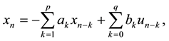
An ARMA model of order (p, q) is considered to have a frequency characterization which is the composite of both forward and backward AR models. This model assumes that the time series {x_n} can be modelled according to the following recursive relationship

(1)

where a_k and b_k are the k-th parameters of the all-pole and all-zero models, respectively, {u_n} is a normalized white noise with distribution and n is the data sample (i.e., 1 £ n £ N). The HOYWE method involves the solution of a set of statistical equations to determine values for the a_k and b_k parameters of this rational model. In this method, only 2p correlation coefficients are involved. It was shown by many researchers, such as Cadzow [9] and Kay [12] , that improved estimates of theses parameters can be obtained by using a larger number of equations than the minimal number (i.e., p) of HOYWE evaluations. This overdetermined set of linear equations can readily be solved by a wide variety of linear algebra techniques, such as least squares, total least squares and singular value decomposition.

Every autocorrelation lag provides property information about the underlying data sequence which is inversely proportional to the lag order. The zero-order lag is proportional to the signal power. The first lag is similar to the correlation between two copies of the signal at adjacent samples in time, and so on. Obviously, as the lag order increases, the provided information becomes less valuable. It is worth noting that estimating a correct model order (i.e., number of equations) is an important issue in signal modelling. Increasing the number of equations is particularly valuable for narrowband processes. In this case, a slow decay of the correlation sequence is expected with relatively large values assigned to higher lag coefficients. For broadband processes, a fast decay of the correlation sequence is expected with little information provided by the higher lag coefficients.

2.2. Singular Value Decomposition

To extract the prerequisite model order values from the overdetermined set of linear equations, the SVD method is often used [17] - [19] . Let A be an m ´ n data matrix with real or complex entries. It is well-known that the following decomposition of A always exists

(2)

where U and V are m ´ m and n ´ n unitary matrices, respectively, p = min(m, n), and S is a rectangular diagonal matrix of the same size as A with real nonnegative entries, {d_i}.These diagonal entries, called the singular values of A, are ordered in descending order of magnitude (i.e.,) with the largest in the upper left-hand corner. The nonzero singular values are the square roots of the eigenvalues of an estimated correlation matrix AA^T or A^TA. Thus, the rank of A equals the number of non-zero singular values. The columns of U and V are the eigenvectors of AA^T and A^TA, respectively.

The pseudo-inverse A^# of Equation (2) is related to the SVD of the matrix A by the formula: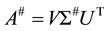, where the diagonal matrix S^# is obtained from S by substituting each positive diagonal entry by its reciprocal. For the SVD computation of a rectangular matrix, highly accurate and numerically stable algorithms were developed [20] - [24] . In the absence of noise, the solution of (2) is often satisfactory. This is because there will be only p nonzero elements in the diagonal matrices S and S^#. The introduction of a small amount of noise tends to change the situation. Some or likely all of the formerly zero singular values of matrix S become small nonzero values. These small diagonal values of S become large diagonal values of S^#, which leads to large perturbations in the estimated LP parameters. This undesirable effect can be minimized by replacing matrix A in the case of noisy data by a lower rank approximation  prior to computation of the LP parameters.

3. Estimation of Noise Variance

In this section, we will first be concerned with the evaluation of the extended order autocorrelation matrix from the higher-order Yule-Walker equations. Then, the SVD method outlined in the previous section is used to compensate for the trivial singular values induced by the AWGN. The resultant AR spectral parameters are subsequently used in the derivation of the noise variance. In the following, the notation a^l and a^h are used to denote AR spectral estimation from LOYWE and HOYWE, respectively, as they provide more understandable descriptions with less information.

As previously stated, the overdetermined modeling method uses more correlations than the minimal number required by the predictor model to establish the normal equations. In this method, the q non-singular higher-order Yule-Walker equations are solved in a least squares sense as specified by

(3)

where the first component is required to be one, and the statistical autocorrelation r_x (n) satisfies the relation:. It was shown in [18] that for N data lengths, a lag indices q of approximately N/2 to

3N/4 provides higher resolution and stable estimates. Accordingly, there exists an inherent trade-off between estimation accuracy and model complexity. Expressing Equation (3) in a compact matrix form gives a set of q linear equations in the p unknowns,

(4)

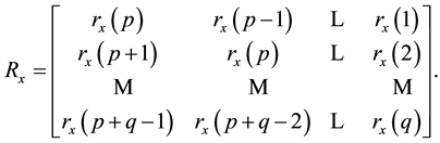
where a^h is the p ´ 1 AR parameter vector, r_x is a q ´ 1 column vector, and R_x denotes the q ´ p ARMA autocorrelation matrix. They are given, respectively, by

(5)

(6)

(7)

Since the autocorrelation lags are unknown, then they may be replaced with estimated autocorrelations using a sample realization of the AR process. However, there is an important issue in AR modelling related to the selection of a suitable autocorrelation lag estimation scheme. The typical unbiased and biased autocorrelation estimates are among the most commonly used techniques in spectral estimation. According to [9] [25] , the former has been proven to be the optimum choice for the lag estimates required in (4). Moreover, the autocorrelation matrix formed from this set of estimates will typically have a desirable Toeplitz structure when using this unbiased scheme. Since only x_n is available, the autocorrelation lags can be generated according to

(8)

The required ARMA model’s AR parameters a^h can be found by solving the q over determined linear equations given in (4). Under noise-free conditions where almost exact autocorrelation lag estimates can be found, the rank of the autocorrelation matrix R_x will be equal to p. Due to noise and a finite data samples, however, there will be inherent statistical errors that will affect the autocorrelation lag estimates. It turns out that R_x will be of full rank, resulting in inaccurate AR parameters estimates. It has been shown that a suitable approach to deal with this problem consists in evaluating the rank-p approximation of the matrix R_x.

As stated previously, SVD is a particularly attractive method for numerically evaluating the rank of a matrix. Let l denotes the rank of the underlying matrix R_x and be its optimum rank-k approximation (assuming k £

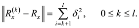
rank [R_x] = l). Having calculated the singular value matrix S from (2), the closest rank-k approximation of the ARMA matrix R_x can be evaluated by the Frobenius norm minimization

(9)

According to (9), the extent to which approximates R_x depends on the sum of the (l - k) smallest singular values squared. In order to measure the validity of this approximation which is independent on the size of the matrix R_x, the best rank-k approximation can be determined by evaluating the following normalized ratio

(10)

The normalized ratio in (10) approaches its maximum value of one as k approaches l. Upon solving Equations (9) and (10), the required ARMA model’s order p can readily be determined, which is set equal to the smallest value of k for which Q_k is evaluated close to one. Thus, the q ´ p matrix of lower rank p that best approximates the underlying ARMA matrix R_x is generated by setting to zero all but the p largest singular values of the matrix S, that is,

(11)

Using this rank approximation approach, the first p singular values of the diagonal matrix S represent the useful data of the matrix R_x whereas the last (l - p) singular values are attributed to noise. Combining Equations (11) and (4) and solving for the ARMA model’s AR parameters gives

(12)

where the matrix designates the pseudo-inverse of. It is generally acknowledged that this overdetermined modeling approach which incorporates the concept of SVD has shown to be worthwhile for performing autoregressive parameter estimates, particularly at lower SNR levels [26] . Upon the determination of the noiseless AR parameters, the noise variance can subsequently be evaluated by the following relationship [27] :

(13)

It is worth noting that the above equation is derived from the least squares analysis of the overdetermined set of p lower-order Yule-Walker equations.

4. Iterative Noise Compensation

In this section, the estimated noise variance is used in an efficient iterative scheme, which is essentially a gradient method, to determine the AR parameters of a lower-order ARMA model with AWGN. The iterative scheme rests on the well-known assumption that in the correlation domain, only the zero-order lag is affected by white noise, while the remain unaffected. The non-singularity of the ARMA matrix is evaluated by considering both the smallest eigenvalue of the autocorrelation matrix and the magnitude of the estimated reflection coefficients.

In order to gain insight into the convergence behavior of the iterative scheme, we define the modulus of the (j + 1)-th reflection coefficient (0 £ j < p) of the matrix R_x and the smallest eigenvalue (in magnitude) as G_j+1 and l_min, respectively. This scheme determines the proportion of noise that should be removed from the zero-order lag so that the matrix R_x is non-singular. Note that the positive-definite property prevents R_x from becoming singular. Upon comparison of either the value of the estimated noise variance to l_min (first criterion) and/or G_j+1 for all j to one (second criterion), the singularity of the matrix R_x can be measured. Providing the value of the estimated noise variance is smaller than the smallest eigenvalue or the estimated reflection coefficients are less than one in magnitude, accurate and stable LP parameters are obtained accordingly. It is worth noting that the second criterion gets only considered when the first one is not satisfied. In this case, the update equation for the entries of the underlying matrix at the ith iteration is given by

(14)

where g is an iteration step size that provides a reasonable tradeoff between the rate of convergence and the estimation accuracy of the autocorrelation matrix [15] , and d (.) is the Kronecker delta. According to the above equation, it can be concluded that the total noisegets subtracted from the zero-order lag if the first criterion is fulfilled, and a fraction otherwise. Considering both criteria, the iterative scheme can then be applied according to the steps shown in Figure 1.

5. Simulation Results

This section presents some computer simulation results which support the thorough analysis presented above. The object of these simulations was to evaluate the effectiveness of the proposed method by comparing its spectral estimation performance with the conventional LMS method (i.e., minimal set of LOYWE evaluations). The first set of experiments involves using LP spectral analysis for estimating the AR model’s parameters. While in the second set of experiments, statistical bias in estimating the AR spectral parameters is achieved.

Designed to be equally intelligible in noise, the sentence “A boy ran down the path” taken from the Hearing in Noise Test (HINT) database [28] and uttered by a male talker was recorded at a sampling rate of 11.025 kHz and used in all the experiments. Figure 2 illustrates the speech waveform given for the two sets of experiments.

As this work is directed towards parametric modeling and analysis of speech, three segments corresponding to vowels, /a/, /e/ and /o/, were selected from the above sentence. Sampled values of white Gaussian noise was generated independently by simulation and added acoustically to achieve an input SNR of roughly 0 dB. These segments are subsequently analyzed with N = 256 data points, p = 15 and p + q = N/2. The iteration step size was optimized through simulation and then set to 0.05. No pre-emphasis was applied on the selected segments. In the following, the proposed method is called a noise compensation based SVD (NCSVD).

Figures 3-5 show the estimated power spectra resulting from the NCSVD and the conventional LMS method, and obtained by averaging 50 realizations for each of the three natural vowels considered in this analysis. We observe from these figures that the formant peaks in the NCSVD spectral estimates are more accurately found and shift towards their right positions. In contrast, the conventional LMS method yields poor spectral estimates at lower SNR levels, as expected.

For each of the three vowels, 50 independent realizations were generated and 300 data points were used from steady-state data to estimate the AR spectral parameters for each realization. Statistical bias in estimating AR parameters is computed by ensemble-averaging over the whole realizations. It is performed on the first four parameters which are related to the first two formant peaks of each of the three vowels. Table 1 summarizes the obtained statistical performance for the given set of vowels. It shows a bias improvement of 0.03, on average, when using the proposed method relative to the conventional LMS. This improvement, however, is achieved at the cost of additional computational effort required for calculating the SVD.

6. Conclusion

For the purpose of AR spectral estimation in additive white Gaussian noise, a robust parametric modelling method was presented which combined an appropriate noise variance estimator with an efficient iterative scheme. The noise-variance estimator was derived from the combination of the ODNE method and the truncated SVD of the autocorrelation matrix. The method provides both accurate and stable LP parameters. It was found from computer simulations that its spectral performance was better than that of the conventional LMS approach in terms of formant peaks tracking. This improvement, however, was achieved at the cost of additional computational effort required for calculating the SVD. Fortunately, there exist extremely efficient and computationally tractable algorithms for speeding up the SVD calculation. Moreover, this extra computational effort should not be a problem given the increasing use of parallel computing architectures in signal processing applications.

Acknowledgements

The authors gratefully acknowledge Teodora Oliveira who participated in a valuable manner in the preparation of this manuscript.

References

- Proakis, J.G., Rader, C.M., Ling, F. and Nikias, C.L. (1992) Advanced Digital Signal Processing. Macmillan Publishing Company, New York.
- Pagano, M. (1974) Estimation of Models of Autoregressive Signal Plus White Noise. The Annals of Statistics, 2, 99- 108. http://dx.doi.org/10.1214/aos/1176342616
- Chakhchoukh, Y. (2010) A New Robust Estimation Method for ARMA Models. IEEE Transactions on Signal Processing, 58, 3512-3522. http://dx.doi.org/10.1109/TSP.2010.2046413
- Kay, S.M. (1979) The Effects of Noise on the Autoregressive Spectral Estimator. IEEE Transactions on Acoustics, Speech and Signal Processing, 27, 478-485. http://dx.doi.org/10.1109/TASSP.1979.1163275
- Dominguez, L.V. (1990) New Insights into the High-Order Yule-Walker Equations. IEEE Transactions on Acoustics, Speech and Signal Processing, 38, 1649-1651.
- Chan, Y.T. and Langford, R.P. (1982) Spectral Estimation via High-Order Yule-Walker Equations. IEEE Transactions on Acoustics, Speech and Signal Processing, 30, 689-698. http://dx.doi.org/10.1109/TASSP.1982.1163946
- Jain, V.K. and Atal, B.S. (1985) Robust LPC Analysis of Speech by Extended Correlation Matching. IEEE International Conference on Acoustics, Speech and Signal Processing, 10, 473-476. http://dx.doi.org/10.1109/ICASSP.1985.1168377
- Jachan, M., Matz, G. and Hlawatsch, F. (2007) Time-Frequency ARMA Models and Parameter Estimators for Underspread Nonstationary Random Processes. IEEE Transactions on Signal Processing, 55, 4366-4376.
- Cadzow, J.A. (1982) Spectral Estimation: An Overdetermined Rational Model Equation Approach. Proceedings of the IEEE, 70, 907-939. http://dx.doi.org/10.1109/PROC.1982.12424
- Izraelevitz, D. and Lim, J.S. (1985) Properties of the Overdetermined Normal Equation Method for Spectral Estimation When Applied to Sinusoids in Noise. IEEE Transactions on Acoustics, Speech and Signal Processing, 33, 406-412. http://dx.doi.org/10.1109/TASSP.1985.1164574
- Jackson, L.B., Jianguo, H., Richards, K. and Haiguang, C. (1989) AR, ARMA, and AR-in-Noise Modeling by Fitting Windowed Correlation Data. IEEE Transactions on Acoustics, Speech and Signal Processing, 37, 1608-1612.
- Kay, S.M. (1980) Noise Compensation for Autoregressive Spectral Estimates. IEEE Transactions on Acoustics, Speech and Signal Processing, 28, 292-303.
- Hu, H.T. (1998) Linear Prediction Analysis of Speech Signals in the Presence of White Gaussian Noise with Unknown Variance. IEE Proceedings on Vision, Image and Signal Processing, 145, 303-308. http://dx.doi.org/10.1049/ip-vis:19982014
- Zhao, Q., Shimamura, T. and Suzuki, J. (2000) Improvement of LPC Analysis of Speech by Noise Compensation. Electronics and Communications in Japan, 83, 73-83.
- Trabelsi, A., Boyer, F.R., Savaria, Y. and Boukadoum, M. (2007) Iterative Noise-Compensated Method to Improve LPC Based Speech Analysis. IEEE International Conference on Electronics, Circuits and Systems, Marrakech, 11-14 December 2007, 1364-1367. http://dx.doi.org/10.1109/ICECS.2007.4511252
- Fattah, S.A., Zhu, W.P. and Ahmad, M.O. (2011) Identification of Autoregressive Moving Average Systems Based on Noise Compensation in the Correlation Domain. IET Signal Processing, 5, 292-305. http://dx.doi.org/10.1049/iet-spr.2009.0240
- Stewart, G.W. (1993) On the Early History of the Singular Value Decomposition. Journal of the Society for Industrial and Applied Mathematics, 35, 551-566. http://dx.doi.org/10.1137/1035134
- Tufts, D. and Kumaresan, R. (1982) Singular Value Decomposition and Improved Frequency Estimation Using Linear Prediction. IEEE Transactions on Acoustics, Speech and Signal Processing, 30, 671-675. http://dx.doi.org/10.1109/TASSP.1982.1163927
- Lee, S. and Hayes, M.H. (2004) Properties of the Singular Value Decomposition for Efficient Data Clustering. IEEE Signal Processing Letters, 11, 862-866. http://dx.doi.org/10.1109/LSP.2004.833513
- Golub, G.H. and Kahan, W.M. (1965) Calculating the Singular Values and Pseudo-Inverse of a Matrix. Journal of the Society for Industrial and Applied Mathematics, 2, 205-224. http://dx.doi.org/10.1137/0702016
- Golub, G.H. and Reinsch, C. (1970) Singular Value Decomposition and Least Squares Solutions. Numerische Mathematik, 14, 403-420. http://dx.doi.org/10.1007/BF02163027
- James, D. and Kahan, W.M. (1990) Accurate Singular Values of Bidiagonal Matrices. SIAM Journal on Scientific and Statistical Computing, 11, 873-912. http://dx.doi.org/10.1137/0911052
- Gu, M. and Eisenstat, S.C. (1995) A Divide-and-Conquer Algorithm for the Bidiagonal SVD. SIAM Journal on Matrix Analysis and Applications, 16, 79-92. http://dx.doi.org/10.1137/S0895479892242232
- Chan, T.F. (1982) An Improved Algorithm for Computing the Singular Value Decomposition. ACM Transaction on Mathematical Software, 8, 72-83. http://dx.doi.org/10.1145/355984.355990
- Tierney, J. (1980) A Study of LPC Analysis of Speech in Additive Noise. IEEE Transactions on Acoustics, Speech and Signal Processing, 28, 389-397. http://dx.doi.org/10.1109/TASSP.1980.1163423
- Cadzow, J.A. (1980) High Performance Spectral Estimation―A New ARMA Method. IEEE Transactions on Acoustics, Speech and Signal Processing, 28, 524-529. http://dx.doi.org/10.1109/TASSP.1980.1163440
- Paliwal, K.K. (1988) Estimation of Noise Variance from the Noisy AR Signal and Its Application in Speech Enhancement. IEEE Transactions on Acoustics, Speech and Signal Processing, 36, 292-294.
- Nilsson, M., Soli, S.D. and Sullivan, J.A. (1994) Development of the Hearing in Noise Test for the Measurement of Speech Reception Thresholds in Quit and in Noise. Journal of the Acoustical Society of America, 95, 1085-1099. http://dx.doi.org/10.1121/1.408469