Open Journal of Yangtze Oil and Gas
Vol.02 No.03(2017), Article ID:77631,15 pages
10.4236/ojogas.2017.23014
Analyses of Nature of Fault through Production Data
Haijun Fan1, Atif Zafar1,2, S. G. Alam2, Muhammad Kashif1, Asif Mehmood1
1China University of Petroleum (East China), Qingdao, China
2University of Karachi, Karachi, Pakistan
Email: petroengineer@126.com, atif_zafar1984@yahoo.com, ghufran_aug27@yahoo.com, 
Copyright © 2017 by authors and Scientific Research Publishing Inc.
This work is licensed under the Creative Commons Attribution International License (CC BY 4.0).
http://creativecommons.org/licenses/by/4.0/


Received: April 7, 2017; Accepted: July 11, 2017; Published: July 14, 2017
ABSTRACT
An application of integration of reservoir production data in analysis for nature of fault is presented in this paper. The real data of a Gas Field (namely RS Gas Field) of L-Basin of Pakistan are used. The basic concept behind this work is to enlighten the importance of production data analysis in a broader way like for finding out the nature of fault i.e. conductive or non-conductive and if it is conductive, what is the leakage factor of the fault etc. Normally in the case of fault analysis we rely on geological and geophysical methods to some extent but in some cases where these geological and geophysical methods are not able to reach any final and firm conclusion because of data limitation or any other reason, production data analysis may play a great role in answering the ambiguities regarding any fault/faults present there. This paper describes the successful implementation of reservoir production data analysis in RS Gas Field where the main uncertainties were identified during initial stage of field development when location of new development well was going to be marked. Numbers and locations of well are important factors of Oil and Gas Filed Developments; but specifically, for Gas Field Development, these factors become more crucial as compared to Oil Field Development; so clear knowledge of any heterogeneity, barrier, boundary or fault is necessary to develop a gas field optimally and economically.
Keywords:
Fault Analysis, Leakage Factor, Production Data, Reservoir Engineering

1. Introduction
The RS concession lies in the L-Basin of Pakistan and in a highly prospective area where the large gas fields of Pakistan are found. The primary objective in this area is the M-Limestone; the secondary objective was the U-Limestone. Both are of early Eocene age. The Late Cretaceous Sandstone provided a tertiary objective. The source rock for the gas is the Lower Cretaceous Shales. Seal for the M-Limestone is provided by the S-Shale, for the U-Limestone, seal is provided by the G-shale.
RS gas field was brought on production in April 2010 with an initial production rate of 16.5 MMscfd gas. Presently (December 2015), the well is producing 14 MMscfd gas, thus showing a decline of 3.24% per year.
After production of more than five years of RS-1 well, the reservoir has been appraised and level of confidence has been increased on initial gas in place estimated through different methods. For further field development, the development well (RS-2) was proposed on the south of the RS-1 (Figure 1) well on the basis of following assumptions and limitations:
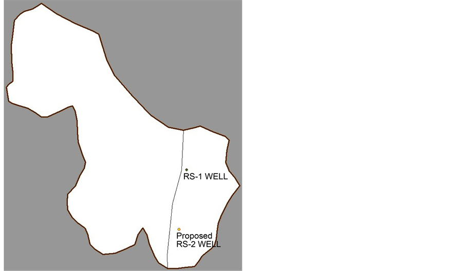
Figure 1. 2D Structure map of RS gas field.
1) The fault near the RS-1 Well is a sealing fault
2) East and West compartment of the reservoir along the fault are not in communication
3) West part may be different reservoir or may not be any reservoir because of lack of seismic data control on that side
The location for RS-2 well was proposed on the basis of some relatively high tops of reservoir. Top of reservoir in RS-1 Well is 1290 m whereas in proposed RS-2 well top of reservoir is 1285 m. It indicates additional 5 m of reservoir in proposed RS-2 well.
2. Methodology
To determine the nature of fault of RS Gas Field Structure, study will be carried
out in two stages. In first stage the pressure and production history will be used in order to calculate initial gas in place of RS Gas Reservoir. This initial gas in place will be verified by volumetric estimation method. If initial gas in place from both the methods is in agreement it will show that dynamic and static methods are on same page that is fault is non-sealing. If it will be the case then further investigation regarding the degree of leakage of fault will be carried out through simulation as shown in Figure 2.

Figure 2. Methodology flow chart.
2.1. Initial Gas In-Place Estimation
This section is concerned with fluid flow in the bulk of the RS Gas Reservoir. The integration of geology and well test analyses will be very helpful [1] . An understanding of the mechanisms controlling fluid displacement will help in maximizing the technically recoverable reserves through
1) Planning reservoir development strategies.
2) Optimizing off take rates at field and reservoir layer level.
3) Marking initial well locations.
4) Designing initial well completions and identifying subsequent interventions.
Knowledge of reservoir drive mechanism is necessary in order to prepare dynamic model to calculate initial gas in-place [2] . Normally, gas reservoirs are produced by expansion of the gas contained in the reservoir. The high compressibility of the gas relative to the water in the reservoir (either connate water or underlying aquifer) makes the gas expansion the dominant drive mechanism. But this depletion drive mechanism changes to water drive mechanism by different indices in different reservoirs depending upon the properties and geometries of the reservoir and aquifer.
To investigate the drive mechanism of RS Gas Reservoir the P/Z Vs Gp Plot (Figure 3) was generated by using the production and pressure history as given in Table 1.

Figure 3. P/Z Vs Gp plot of RS gas reservoir.

Table 1. Pressure and production history of RS gas field.
For a volumetric reservoir, the relationship between (P/Z) and Gp is essentially linear because of volumetric depletion of gas reservoir and by extrapolation of the straight line to abscissa, i.e., at P/Z = 0, gives the value of the gas initially in place as G = Gp [3] . But the graphical representation of pressure and production history of RS Reservoir shows the presence of water influx, as shown Figure 1 where the plot of (P/Z) versus Gp deviates from the linear relationship, it indicates the presence of water encroachment [4] [5] .
After confirming by P/Z Vs Gp plot that there is water encroachment in the reservoir [6] [7] , the next step is to generate the Cole plot which is more sensitive reservoir drive mechanism diagnostic plot [8] .
Cole plot of RS Gas Reservoir (Figure 4) shows that reservoir has water drive mechanism means it is has some degree of pressure maintenance due to water encroachment into the reservoir from the aquifer. After validation of reservoir drive mechanism now the question arises about the strength of aquifer support. Accurate aquifer modeling will be done in next step by verifying the history matching and production and pressure simulation. If the comparison of P/Z Vs Gp plot (Figure 3) and Cole plot (Figure 4) is made with their benchmark plots (Figure 5) it reveals that RS Gas Reservoir has moderate water dive support or in other words it has partial water drive mechanism.
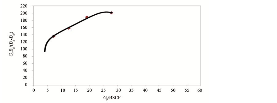
Figure 4. Cole plot of RS gas reservoir.
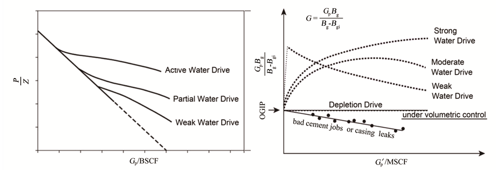
Figure 5. General shapes of P/Z Vs Gp and Cole plot as a function of aquifer strength.
Material Balance Method is adopted to estimate the initial gas in place of Jin Gas Reservoir by using the pressure values obtained by well test interpretation using the commercial software. The material balance is based on the principle of the conservation of mass:
Mass of fluids originally in place = Fluids produced + Remaining fluids in place.
The material balance program uses a conceptual model of the reservoir to predict the reservoir behavior based on the effects of reservoir fluids production [9] . The material balance equation is zero-dimensional, meaning that it is based on a tank model and does not take into account the geometry of the reservoir, the drainage areas, the position and orientation of the wells, etc [10] . However, the material balance approach proved to be a very useful tool in this study in performing many tasks i.e. in quantifying different parameters of a reservoir such as hydrocarbon in place, in determining the presence, the type and size of an aquifer, encroachment angle, etc., in predicting the reservoir performance and manifold back pressures for a given production schedule and also in predicting the reservoir performance and well production for a given manifold pressure schedule [11] [12] .
Havlena-Odeh graphical method was adopted to perform material balance calculations which matched with Hurst-Everdingen Dake Radial Aquifer model [13] [14] [15] . An iterative non linear regression was used to automatically find the best mathematical fit for a given model showed original gas in place of 104 BSCF (Figure 6).
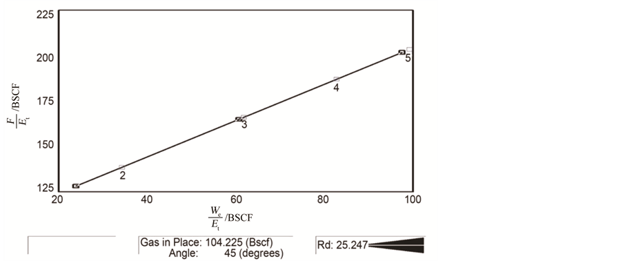
Figure 6. Havlena-odeh graphical method of material balance.
Reservoir Driver Mechanism indices are also calculated and plotted (Figure 7) which translates current average water saturation as 56.6%, which was 48.7% at initial condition. Initial water drive index was 25% but now it is 50%, which means gas expansion within the reservoir has reduced to 50%.
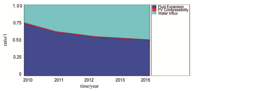
Figure 7. RS gas reservoir drive indices.
Material balance estimates are also validated by history matching of production and pressures which showed good match (Figure 8). A simulation of production is run to check the validity of the results. Gas and water relative per- meabilities are estimated from historical WGR.
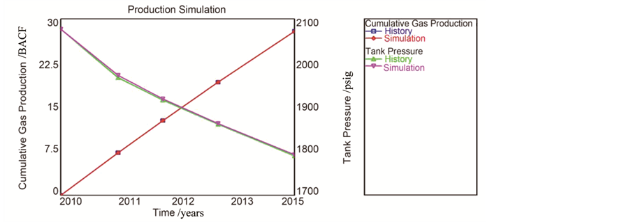
Figure 8. RS gas reservoir production and pressure simulation.
The accurate and perfect history matching is achieved through simulation which indicates the authenticity and validity of results of different parameters of reservoir as well as aquifer [16] . The models which are used for reservoir and aquifer are correct and the set of pressure used in this modeling also has been proved accurate. This set of pressure has been obtained through the well testing interpretation. As per the matched material balance dynamic model, the yearly water encroachment into the reservoir is given in Table 2. The cumulative water production into the reservoir is estimated 23 MMRB. The corrected P/Z Vs Gp plot has been generated manually too by using Microsoft Excel as shown in Figure 9. In this corrected P/Z Vs Gp plot volume of encroached water is incorporated and subtracted.
The Initial Gas In-Place of RS Gas Field calculated by Material Balance is also verified by Volumetric Reserve Estimation Method. Volumetric Method uses
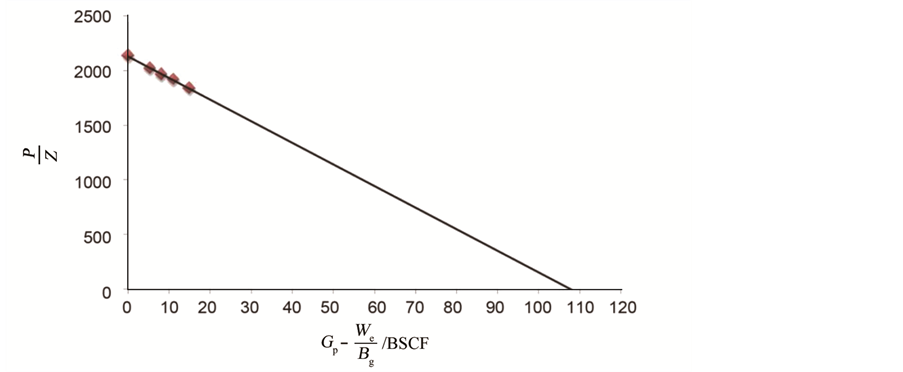
Figure 9. Corrected P/Z vs Gp plot of RS gas reservoir.
Table 2. Pressure, gas production and water encroachment of RS gas field.
static properties of the reservoir and Material Balance Method is the dynamic model of the reservoir [17] . The following two approaches are used to calculate the IGIP of RS Gas Field.
Firstly the reservoir is considered as rectangular in shape (Figure 10) as classical Reservoir Engineering and petro-physical model employ in the following renowned equation.

Figure 10. Rectangular reservoir.
 (1)
(1)
where G means gas in place (SCF), A is reservoir area (acres), h shows reservoir thickness (feet), θ indicates porosity (fractions), Swi is water saturation (fractions) and Bgi is gas formation volume factor (ft3/SCF). NTG in the Figure 10 stands for Net to Gross ratio of thickness
By using Equation (1)


Volumetric Method of initial gas in place calculation incorporates subsurface and Isopachous map. These maps are generated on the basis of data collected from seismic surveys, coring, wire-line logging and different types of well testing. Basically subsurface contour map demonstrates the lines connecting points of same elevations of a geologic structure whereas a net Isopachous map demonstrates lines connecting points of identical net formation thickness. Isopach lines are the individual lines connecting points of identical thickness. These maps are employed to estimate the productive bulk volume of the reservoir. When there is Oil-Water, Gas-Water and/or Oil-Gas contact, the contour map is used in generating the Isopachous maps. The zero isopach line shows the contact line. By planimetering the areas between the Isopachous lines the volume of the whole reservoir is estimated therefore there are many problems in generating these maps because it requires the accurate finding of net thickness from the wire-line logs interpretation and the boundary of the reservoir productive area as highlighted by the Oil-Water, Gas-Water and/or Oil-Gas contacts, permeability barriers and/or faults on the subsurface contour map.
To calculate the volume of the reservoir productive zone two equations are commonly used. The volume of the frustum of the pyramid is estimated by
 (2)
(2)
where ΔVb shows the reservoir bulk volume (acre-feet), An shows the area occupied by lower isopach line (acres), An+1 shows the area occupied by the upper isopach line (acres) and h represents the interval between the isopach lines (feet) as shown in Figure 11.

Figure 11. Isopachous map and cross section of an idealized reservoir, Craft B. C (1994).
Equation (3) is used to calculate the volume between successive isopach lines [18] . The total volume is the sum of these individual volumes. The trapezoidal volume is given by:
 (3)
(3)
Or for a sequence of consecutives trapezoids
 (4)
(4)
For the excellent accuracy pyramidal formula is used because of its simpler form, however, the trapezoidal formula is also generally used. The trapezoidal formula normally brings in an error of 2% when the ratio of consecutive areas is equal or less than to 0.50. Therefore, a commonly accepted rule is that wherever the ratio of areas of any two consecutive lines is less than 0.5, the pyramidal formula is used. Whenever the ratios of the areas of any two consecutive lines is found to be greater than 0.5, the trapezoidal formula is used as shown in this case of RS Gas Field in Table 3.
Table 3. Contour-wise area and volume calculation by using shape factor.
By using Equation (1):


By using this technique to calculate the initial gas in place, a more accurate number of 106 BSCF is estimated. The all other geological input parameters are same as the previous method where reservoir was assumed as a rectangular shape reservoir.
2.2. Numerical Simulation
To verify the initial gas in-place estimation of RS Gas Field calculated by different methods earlier, Numerical Simulation has also been carried out by developing a 3D static and dynamic reservoir model in a commercial simulator.
RS Gas Reservoir has been divided into seven zones/layers on the basis of petro-physical properties i.e. porosity permeability and net to gross ratio (shale content) in order to achieve accurate results from numerical simulation model. Figure 12 shows the layering of RS Reservoir on the basis of porosity which is calculated from well logs. Model reveals that two bottom zones are more porous than other zones.
Each zone of RS Gas Reservoir has also been assigned by different values of permeabilities which were estimated through well logs interpretation as shown in Figure 13. Since on well logs there is no clear evidence of sharp vertical gas- water contact but material balance model and history matching shows some pressure maintenance through water encroachment therefore it was concluded that this reservoir has edge water drive mechanism.

Figure 12. Porosity variation in layers of RS reservoir.

Figure 13. Permeability variation in layers of RS reservoir.
After putting all the required information of RS Gas Reservoir and RS-1 Well in the simulator in order to verify the initial gas in place of the field, simulation was successfully run and achieved logical results having greater level of confidence. Model in Figure 14 shows the current situation of pressure distribution of the reservoir after production of almost six years. The IGIP translated from this simulation model is 102 BSCF which is in fully agreement with all the other methods of gas in place calculations adopted previously.
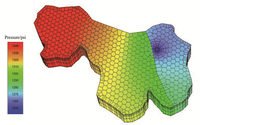
Figure 14. Pressure distribution of RS reservoir on current condition.
Simulation results (Table 4) confirm the Initial gas in place estimation through Volumetric Method and Material Balance Method which are based upon the parameters (mainly Pressure) obtained by well testing interpretation of RS Gas Field.
Table 4. Summary of input and results of numerical simulation.
Now after applying different methods and techniques of Reservoir Engineering it can be summarized that results from each method validate the outcomes of other methods. The Figure 14 is the graphical representation of comparison of IGIP estimation results of RS Gas Field through different methods. They are all in agreement with each other and confirm that fault is conductive.
Now after applying different methods and techniques of Reservoir Engineering it can be summarized that results from each method validate the outcomes of other methods.
Figure 15 is the graphical representation of comparison of IGIP estimation results of RS Gas Field through different methods. They are all in agreement with each other and confirm that fault is conductive.
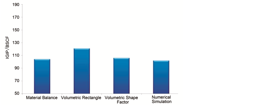
Figure 15. Comparison of IGIP estimation through different methods.
2.3. Sensitivity Analyses
Now the next step is to find the degree of leakage or in other words the leakage factor of fault. For this different cases are run by setting the different values of leakage factor of the fault as an input of the model. In output cumulative produced gas is little bit different against each input value of the leakage factor of the fault. Since the cumulative produced gas is a known factor so it is matched with the correct input value of leakage factor of the fault
Table 5 shows the results of sensitivity analyses for fault leakage factor. Since in this case of RS Gas Reservoir there is only one well therefore there is lack of control on average pressure too. The western portion of the reservoir has no recorded pressure therefore gas production is the main matching factor in this case and average reservoir pressure is output, otherwise, in general, average reservoir pressure may also be used to match to increase the confidence level on results of leakage factor. Gas Production of simulation run number 7 is well matched so leakage factor 0.4 of this run is the simulated output.
Table 5. Summary of input and results of numerical simulation sensitivity analyses.
3. Conclusion
This is a complete comprehensive algorithm of using and validating the different methods, tools and techniques of Geology and Reservoir Engineering in order to investigate nature of any fault. Firstly material balance was carried out by using pressures obtained from well testing interpretation then volumetric method was applied considering the whole reservoir as a single compartment/pool. Although outputs from both methods were in agreement, numerical simulation was also done to further firm the output from these two methods. In the end, unique technique was adopted to match the leakage factor of the conductive fault. Hence the ambiguity regarding well location which was marked only on geological and geophysical data can be cleared now by looking at the detailed fault analyses using dynamic production data. Now the proposed RS-2 well can be located at western part of the structure without any fear. This is not only the matter of location, in fact it belongs to economics also. The methodology given in this research proved to be very helpful in the reservoir study of RS Gas Field and it may open the new windows for further research in this direction.
Cite this paper
Fan, H.J., Zafar, A., Alam, S.G., Kashif, M. and Mehmood, A. (2017) Analyses of Nature of Fault through Production Data. Open Journal of Yangtze Gas and Oil, 2, 176-190. https://doi.org/10.4236/ojogas.2017.23014
References
- 1. Corbett, P., Zheng, S.-Y., Pinisetti, Moe, Mesmari and Abdallah (1998) The Integration of Geology and Well Testing for Improved Fluvial Reservoir Characterization. Heriot-Watt University.
- 2. Agarwal, R.G., Al-Hussainy, R. and Ramey Jr., H.J. (1965) The Importance of Water Influx in Gas Reservoirs. Journal of Petroleum Technology, 17, 1336-1342.
https://doi.org/10.2118/1244-PA - 3. Brownscombe, E.R. and Collins, F. (1949) Estimation of Reserves and Water Drive from Pressure and Production History. Journal of Petroleum Technology, 1, 92-99.
https://doi.org/10.2118/949092-G - 4. Bruns, J.R., Fetkovich, M.J. and Meitzen, V.C. (1965) The Effect of Water Influx on p/z-Cumulative Gas Production Curves. Journal of Petroleum Technology, 17, 287-291.
https://doi.org/10.2118/898-PA - 5. Chierici, G.L.P.G. and Ciucci, G.M. (1967) Water Drive Gas Reservoirs: Uncertainty in Reserves Evaluation from Past History. Journal of Petroleum Technology, 19, 237-244.
https://doi.org/10.2118/1480-PA - 6. Ikoku, C.U. (1984) Natural Gas Reservoir Engineering. John Wiley & Sons, New York.
- 7. Ismadi, D., Suthichhoti, P. and Kabir, C.S. (2010) Understanding Well Performance with Surveillance Data. Journal of Petroleum Science & Engineering, 74, 99-106.
https://doi.org/10.1016/j.petrol.2010.08.015 - 8. Tarek, A. (2006) Reservoir Engineering Handbook. Elsevier.
- 9. Archer, J.S. and Wall, C.G. (1986) Petroleum Engineering Principles and Practice. Graham and Trotman.
- 10. Bingguang, H. (1998) Practical and Dynamic Analysis of Reservoir Engineering. Petroleum Industry Press, Beijing.
- 11. Shi, L.L. (2000) Natural Gas Engineering. Petroleum Industry Press, Beijing.
- 12. Yuan, Q.C. (1997) Reservoir Engineering Calculations. Petroleum Industry Press, Beijing.
- 13. Carter, R.D. and Tracy, G.W. (1960) An Improved Method for Calculating Water Influx. American Invitational Mathematics Examination, 219, 415-417.
- 14. Havlena, D. and Odeh, A.S. (1963) The Material Balance as an Equation of a Straight Line. Journal of Petroleum Technology, 15, 896-900.
https://doi.org/10.2118/559-PA - 15. Hurst, W. (1943) Water Influx into a Reservoir and Its Application to the Equation of Volumetric Balance. American Invitational Mathematics Examination, 151, 57-72.
https://doi.org/10.2118/943057-g - 16. Dake, L.P. (1994) The Practice of Reservoir Engineering. Elsevier, Amsterdam.
- 17. Zafar, A. and Fan, H. (2017) Combination of Geological, Geophysical and Reservoir Engineering Analyses in Field Development: A Case Study. International Journal of Environmental, Chemical, Ecological, Geological and Geophysical Engineering, 11, 36-43.
- 18. Craft, B.C., Hawkins, M.F. and Terry, R.E. (1959) Applied Reservoir Engineering. Prentice Hall, Upper Saddle River.