International Journal of Geosciences
Vol.5 No.6(2014), Article ID:45948,11 pages DOI:10.4236/ijg.2014.56056
Relevance of AEM and TEM to Detect the Groundwater Aquifer at Faiyum Oasis Area, Faiyum, Egypt
A. A. Basheer1*, A. I. Taha1, A. El-Kotb1, F. A. Abdalla2, S. O. Elkhateeb2
1Geomagnetic and Geoelectric Department, National Research Institute of Astronomy and Geophysics, Cairo, Egypt
2Geology Department, Faculty of Science, South Valley University, Qena, Egypt
Email: *alhussein.adham.basheer.mohammed@gmail.com
Copyright © 2014 by authors and Scientific Research Publishing Inc.
This work is licensed under the Creative Commons Attribution International License (CC BY).
http://creativecommons.org/licenses/by/4.0/


Received 23 March 2014; revised 19 April 2014; accepted 6 May 2014
ABSTRACT
This study investigates the groundwater aquifer located in Fayuim oasis. In this study, two of the electromagnetic measurement methods have been used in determining the hydrological situation in the Fayoum oasis. The first is airborne electromagnetic (AEM) which, sometimes is referred to as Helicopter electromagnetic (HEM) and the second is ground Time-domain Electromagnetic method (TEM). The subsurface consists of four geoelectrical layers with a rough slope towards the center. The third and the fourth layers in the succession are suggested to be the two-groundwater aquifers. The third layer saturates with fresh water overlying saline water which exists in the bottom of the second one. It is worth mentioning that the depth of the fresh water surface undulates between the surface level in two lakes in the study area and 57 meters below the ground, whereas the thickness of the fresh water aquifer varies from 13 to 36 meters. The depth of the saline water surface undulates between 59 and 81 meters below the ground. In general, airborne electromagnetic surveying has the advantage of fast resistivity mapping with high lateral resolution. Groundbased geophysical surveys are often more accurate, but they are definitely slower than airborne surveys. It depends on targets of interest, time, budget, and manpower available by the method or the combination of methods that will be chosen. A combination of different methods is useful to obtain a detailed understanding of the subsurface resistivity distribution.
Keywords
Airborne Electromagnetic [Frequency-Domain], Ground Electromagnetic [Time-Domain] AEM, TEM, Hydrogeophysics, Al Faiyum Oasis/Lake, Egypt

1. Introduction
Al Faiyum Oasis area covers an area of about 90 km2. It lies between latitudes 29.505 and 29.3025 N and longitudes 30.2855 and 30.5445 E (Figure 1). Generally, Faiyum area is considered as a depressed area in the western desert of Egypt. It takes its water from both River Nile in the east and from seasonal rainfalls. The main target of the study is to shed light on the delineation of the groundwater, its ability to be used, and its extraction to help in living and farming activities. We use two geophysical tools and compare between its results to draw the isopach map of the water aquifer. The first method is airborne electromagnetic or helicopter electromagnetic method. The second is Ground Time domain electromagnetic method. Both methods have the same basic concept. It is obvious that the first method is faster and time-saving while the second is slow and time-consuming.
2. Geological Setting
2.1. Surface Geology
Said [1] , in describing the tectonic framework of Egypt, concluded that the country is composed of three structural units: the Arabo-Nubian massif, the stable shelf, and the unstable shelf. The Arabo-Nubian massif is the basement core, and these rocks are well exposed east of the Faiyum in major ranges of the southern Sinai and along the Red Sea in the East Desert of Egypt.
The Arabo-Nubian massif is overlapped and surrounded by the stable shelf, an area of thin continental and epi-continental Cretaceous and Cenozoic units. The Upper Cretaceous-Lower Tertiary shallow-water Nubian Sandstone is overlaid by Eocene rocks, part of which were investigated in this study. The Eocene shale, limestone, and sandstone represent a major marine transgression that covered the stable shelf. The transgression of the sea began near the Late Cretaceous-Early Tertiary transition and ended with a regression that took place from the Middle Eocene to near the close of the Oligocene.
The stable shelf, according to Said [1] , is characterized by the thinness of the sedimentary section, minor normal faulting, and the basin producing rift zones of the Red Sea-Suez region. Although major anticline features are lacking in the stable shelf, there are several domes that have broad and gentle flanks on all sides. Minor movement of these structures has produced local disasters rather than major unconformities.
The Faiyum area lies within Said’s stable shelf. Areas west of Gebel el-Rus and the Nile-Faiyum divide, in the West Desert of Egypt, have been extensively faulted and folded. To the east, the Nile valley is also fault controlled. The Faiyum depression and its surrounding escarpments, however, have escaped the effects of major faulting and folding. Gebel el-Rus area lacks any significant faults, but minor tilting of Eocene strata is apparent.
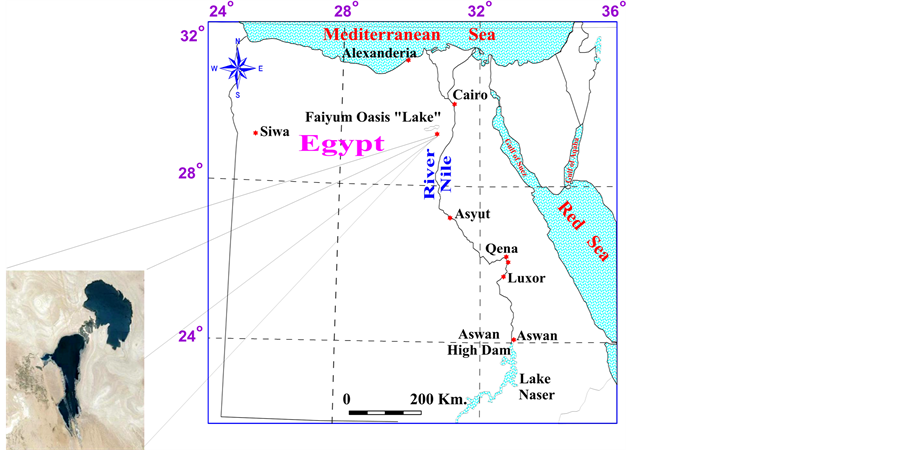
Figure 1. Location map of the study area.
A gentle northward dip of 3 degrees to 8 degrees of Middle and Upper Eocene rocks produced a subtle but observable angular unconformity between these rocks and overlying, essentially horizontal, Pliocene deposits. According to Tamer [2] and [3] , the Faiyum depression overlies the axis of a major anticline and is affected by normal faulting. He described a great monocline edge that bounds the depression on the northern and eastern sides (Figure 2).
2.2. Stratigraphy
The stratigraphic units at some localities of the study area were studied by Said [1] and Tamer [2] and [3] . Middle Eocene, Upper Eocene, and Oligocene rocks crop out in the mapped area. Several classifications are proposed for the Eocene rocks in the different parts of the study area. Table 1 shows the most-accepted classifications of Al Faiyum Lake and the study area.
3. Applied Geophysical Methods
3.1. Instrumentation for Airborne EM Surveys
Electrical and electromagnetic (EM) methods both provide information about the subsurface resistivity distribution.
As in Direct Current (DC) electrical methods, current is injected directly into the subsurface that are limited to

Table 1. Eocene rock units of Al Faiyum Lake (modified from Tamer [2] and [3] ).
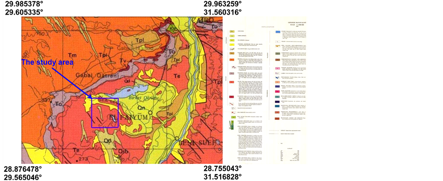
Figure 2. Geologic map of 15th May area, compiled from the geological survey of Egypt (1983) and Conoco Coral (1987).
be applied on the ground.
On the contrary, EM methods are based on the propagation of EM fields, which induce currents in the subsurface and therefore both ground-based and airborne EM measurements are feasible. A successful application of DC and EM methods for differentiating subsurface resistivity structures requires a sufficiently large resistivity contrast between the target and the surrounding material.
Air-Borne Electromagnetic (AEM)
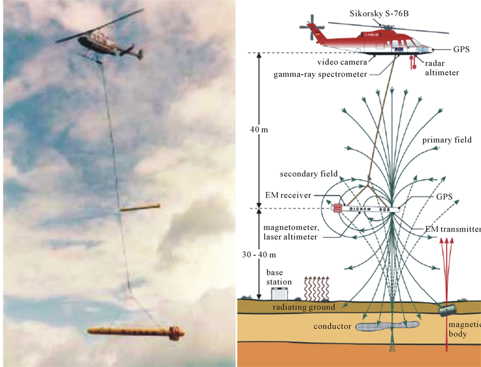
AEM systems Figure 3(a) utilizes several transmitter and receiver coils simultaneously. The transmitter signals and the primary magnetic fields are generated by sinusoidal current flow through the transmitter coils at discrete frequencies. The oscillating primary magnetic fields induce eddy currents in the subsurface. These currents generate the secondary magnetic fields, which depend on the conductivity distribution of the subsurface. The secondary magnetic fields measured by the receiver coils are divided by the primary magnetic fields expected at the centre of the receiver coils and the ratio is measured in parts per million. As the secondary fields are very small with respect to the primary fields, the primary fields have to be bucked. The orientation of the transmitter coils is horizontal or vertical and the receiver coils are oriented in a maximum coupled position resulting in horizontal coplanar, vertical coplanar or vertical coaxial coil systems. Typically 4 - 6 frequencies are used on modern AEM systems [4] .
Compared to ground based EM systems, the vertical distance from the TX-RX system to the target is large. This makes the in-phase and quadrate anomalies quite small. The value of the secondary field is typically measured in parts-permillion (ppm) of the primary magnetic field. Digital helicopter-borne electromagnetic (DIGAEM) survey type has been used in this study.
Bucking coil used to suppress the primary magnetic field at the RX. This allows a weak secondary field to be detected in the presence of a strong primary field. Multiple coil configurations are used. This allows 9 combinations of TX and RX to be used. These will couple differently with different conductor geometries. Multiple frequencies give estimate of depth variation of conductivity [5] .
Depth of penetration depends on TX-RX distance, frequency and the skin depth. It is clearly noted that the measuring of weak secondary magnetic fields in the presence of the primary magnetic field is difficult. Very strong conductors have small quadrature response. Thus, the best targets in mineral exploration and structure mapping are the most difficult to detect with frequency domain EM. Multiple frequencies can be used to estimate conductivity with depth variations. The measured data displayed as secondary field/primary field as ppm or as ground (terrain) conductivity/resistivity map as in 2D.
The AEM system operates at five frequencies are ranging from 56 Hz to 192 kHz. The transmitters and receivers of the horizontal coplanar coil system are about 6.7 m apart. GPS provide the positions of the helicopter and the system. Laser and radar altimeters record the altitudes of the AEM system and the helicopter, respectively. The nominal ground clearance of the system is 30 - 40 m. The sampling rate of 10 Hz provides sampling distances of about 4 m at a flight velocity of 140 km/h.
To interpret the AEM data in terms of layered-earth resistivity models the Marquardt-Levenberg 1-D inversion technique [6] and [7] is used.
3.2. TEM Sounding Method
Transient sounding is typically made using non-grounded squared loops for transmitter and receiver antennas. The steady transmitter current produces a primary magnetic field, which is directed upward inside the loop and downward outside the loop. When the transmitter current is abruptly turned off, current is induced in the ground, which tries to maintain the magnetic field, which is presented prior to turn off. The magnetic field produced by the induced current is called the secondary magnetic field. The induced current will flow in horizontal circles under the transmitter loop.
Initially, the current is concentrated near the surface, but as time passes the maximum current density moves downward and outward [8] . The diffusion and dissipation of the current density are controlled by the resistivity of the ground. The more resistive the ground, the faster the maximum current diffuses downward, and the more rapid the dissipation of the current. For a loge red earth, the current will reside longer in conductive zones than in resistive zones of similar thickness [9] .
Because the induced current is controlled by the resistivity structure of the material beneath the loop, the
 (a)
(a)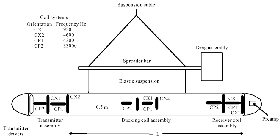 (b)
(b)
Figure 3. (a) Helicopter electromagnetic system; (b) BGR system: The nominal bird altitude is 30 - 40 m above the ground. The helicopter is also equipped with differential GPS, video camera and a radar-altimeter; (c) The system of HEM (called the bird).
secondary magnetic field produced by this current system can be measured to determine the geoelectrical section [10] and [11] .
3.2.1. Time-Domain Electromagnetic Conductivity Meter
SIROTEM MK3 instrument, which is made in Australia, is used in this study. SIROTEM stands for Scientific Industrial Research Organization TEM. SIROTEM MK3 detects underground conducting materials by transmitting electrical pulses along loops of cable laid out on the surface. It is unique in having the transmitter and receiver in a single unit. The major components of SIROTEM MK3 are contained in a robust and portable console unit.
3.2.2. Physical Basis of TEM Sounding
TEM soundings are made with a receiver and transmitter unit attached to a receiver and a large transmitter loop. The transmitter passes a constant current through the loop, which produces a primary magnetic field Figure 4. The current is quickly turned off there by interrupting the primary magnetic field. To satisfy Faraday’s law, currents are induced in the ground, which instantaneously maintain the primary magnetic field. This current system, which flows in closed paths below the transmitter loop, produces a secondary magnetic field. Changes of the secondary magnetic field with time induce a voltage in the receiver, because the magnitude and distribution of the current intensity depend upon the resistivity of the ground. The voltage gives information about the resistivity of the ground. The locus of the maximum amplitude of the induced currents diffuses downward and outward with time, thereby giving information about deeper regions as time increases [8] . The signal recorded by the receiver is called a transient.
4. Data Interpretation
4.1. AEM (Frequency Domain) Data Processing
The aim of the data processing is to extract those field values from the measured data that correspond to the subsurface material parameters and to eliminate—or at least to minimize—those portions in the data that are affected by sources not belonging to the subsurface. AEM data processing requires a number of processing steps such as the conversion of measured voltages to relative secondary field values using calibration signals, standard and advanced drift corrections (zero-level drift correction/2D leveling), and other necessary data corrections [12] [13] .
The AEM system is calibrated using external and internal calibration coils, which produce definite signals in
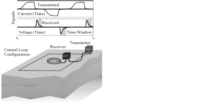
Figure 4. TEM system in central-loop configuration and the transmitted and received TEM waveforms.
the AEM data measured. The external coils are used for the calibration on ground in order to derive the conversion factors. After phase and gain adjustment at the beginning of each survey flight. The calibration is checked using internal calibration coils several times during a survey flight. Phase and gain adjustments are best performed above highly resistive ground or at high flight altitude (e.g. 350 m).
The signals measured at high altitude are due to insufficiently bucked-out primary fields, coupling effects with the aircraft, or (thermal) system drift. These values are used to shift the AEM data with respect to their zerolevels. The zero leveling eliminates the long-term quasi-linear drift; the affect of short-term variations, however, caused by e.g. varying air temperatures due to varying sensor elevations cannot be corrected successfully by this procedure. 2D filter techniques (micro-leveling) are necessary to adjust the line data in order to remove the stripe patterns resulting from remaining zero-level and calibration errors.
As the dependency of the secondary field on both the resistivity of the subsurface and the sensor altitude is strongly non-linear, the half-space parameters are leveled instead. The secondary field components are then leveled with respect to synthetic AEM data derived from the leveled half-space parameters [4] .
External sources (e.g. radio transmitters or power lines) or strong man-made conductors affect the AEM data. Noise can be eliminated from the AEM data by appropriate filtering or interpolation procedures. The elimination of induction effects from buildings and other electrical installations or effects from strongly magnetized sources is a very sensitive processing step as these effects are often not clearly separable from that of natural sources.
4.2. Calculation of Resistivity Models
From the three electric and magnetic material parameters, electrical conductivity, dielectric permittivity, and magnetic permeability describe the electromagnetic properties of the subsurface. The conductivity dominates the AEM measurements in most cases, while permittivity and permeability have only a minor influence at high and low frequencies, respectively. Thus, the conductivity or its inverse (the resistivity) is commonly modeled to explain the AEM data.
Resistivity models are generally derived from the secondary field data (in-phase and quadrature) using automatic inversion procedures as the huge number of data values available in airborne surveys is hardly processable by manual modeling. Therefore, simple resistivity models, the homogeneous half-space and the layered halfspace, are used. While the homogeneous half-space inversion uses single frequency data, multi-layer (one-dimensional, 1-D) inversion takes the data of all frequencies into account. Beard [14] and Siemon [15] compared a number of approaches available for calculating the AEM half-space parameters, the apparent resistivity qa [Xm] and the corresponding centroid depth [Zm]. Half-space parameters obtained for a number of frequencies enable the presentation of the AEM results as apparent resistivity maps [16] resolving different depths or apparent resistivity/depth sections [17] and [18] . There are also several procedures available for the layered half-space inversion of AEM data which are often adapted from algorithms developed for ground-based EM data. A comparison of several 1-D inversion procedures is presented by [19] . In this paper, the procedures described by [7] are used.
4.3. AEM (Frequency Domain) Data Interpretation
Al Faiyum site inversion procedure requires a starting model that is derived from apparent resistivity vs. centric depth values. This initial multi-layer resistivity-thickness model is fitted to the AEM data using sensitivities (Jacobian matrix) that are calculated analytically. The inversion procedure is stopped when a given threshold is reached. This threshold is de-fined as the differential fit of the modeled data to the measured AEM data, i.e. the inversion stops when the enhancement of the fit is less than e.g. 10%.
4.4. Ground TEM (Time Domain) Data Processing
There are many ways in which TEM data can be processed and these are largely dependent upon which instrument system is used to acquire the original data. Most TEM systems record the transient voltage at a number of discrete intervals during the voltage decay, after the applied current is switched off. In each time, the current is applied and then stopped, measurements are taken; when the current is applied again and switched off, a repeat set of measurements is taken. This process may be repeated many tens of times at a given location with all the data are being logged automatically. Consequently, these many data can be processed to improve the signal-tonoise ratio. At the same time, the field data are checked for repeatability. Commonly, the data are normalized with respect to the transmitter current or other system parameter, and the effects of the time decay may be amplified in compensation by normalizing the observed field at each point with the respective primary field value at the same point.
[20] described a data processing sequence for long offset transient EM’ (LOTEM) sounding undertaken in Germany. Three data processing stages were formulated:
1) Pre-stack processing, was used to remove unwanted periodic noise using filtering such as a notch to remove noise associated with AC power lines. A selective stacking algorithm was applied to average only a percentage of the data around the median of the individual time samples. The consequence of this was to reduce the noise content [21] .
2) The post-stack processing was to apply a slight time variable smoothing filter. The culmination of this processing was the production of logarithmic plots of apparent resistivity as a function of decay time.
A variety of plots of processed data can be produced, such as transient decay (logarithmic) plots of voltage (in mV) versus decay time (in msec), response profiles (graphs of measured voltage at a selected decay time at all stations in a survey area); response contours (the response profile data plotted in map form) and apparent resistivity plots, either as profiles or maps.
Interpretation methods are as varied as the different types of data plots and systems used to acquire the data. Typically, the interpretation is undertaken in two stages:
1) The first is to locate a possible sub-surface target on the basis of the shape, size and location of the anomalies evident on profiles and maps of relevant parameters.
2) The second, more quantitative, stage is to determine the quality of the conductor using time constants determined from decay plots of the field intensity at one or more locations.
Various types of display parameter are useful for different applications. For example, apparent resistivity soundings can be extremely useful in hydrogeological investigation and in geological mapping but they provide very little information appropriate for mineral exploration.
In this study, we carried out TEM soundings 49 stations as a regional study in all the study area using a SIROTEM time-domain system with 50 m × 50 m loop as a transmitter and receiver at the same time. The used delay times are in the range 20 ms to 40 ms, and we used the TEMIXXL [22] software (Interpex Ltd., USA) in interpretation. Figure 5 shows an example of TEM sounding interpretation result.
5. Results, Discussion and Conclusion
Results of each of the two used methods are compared. Figure 6 shows the resistivity maps for the study area in

Figure 5. Example of interoperation of TEM sounding No. 12.
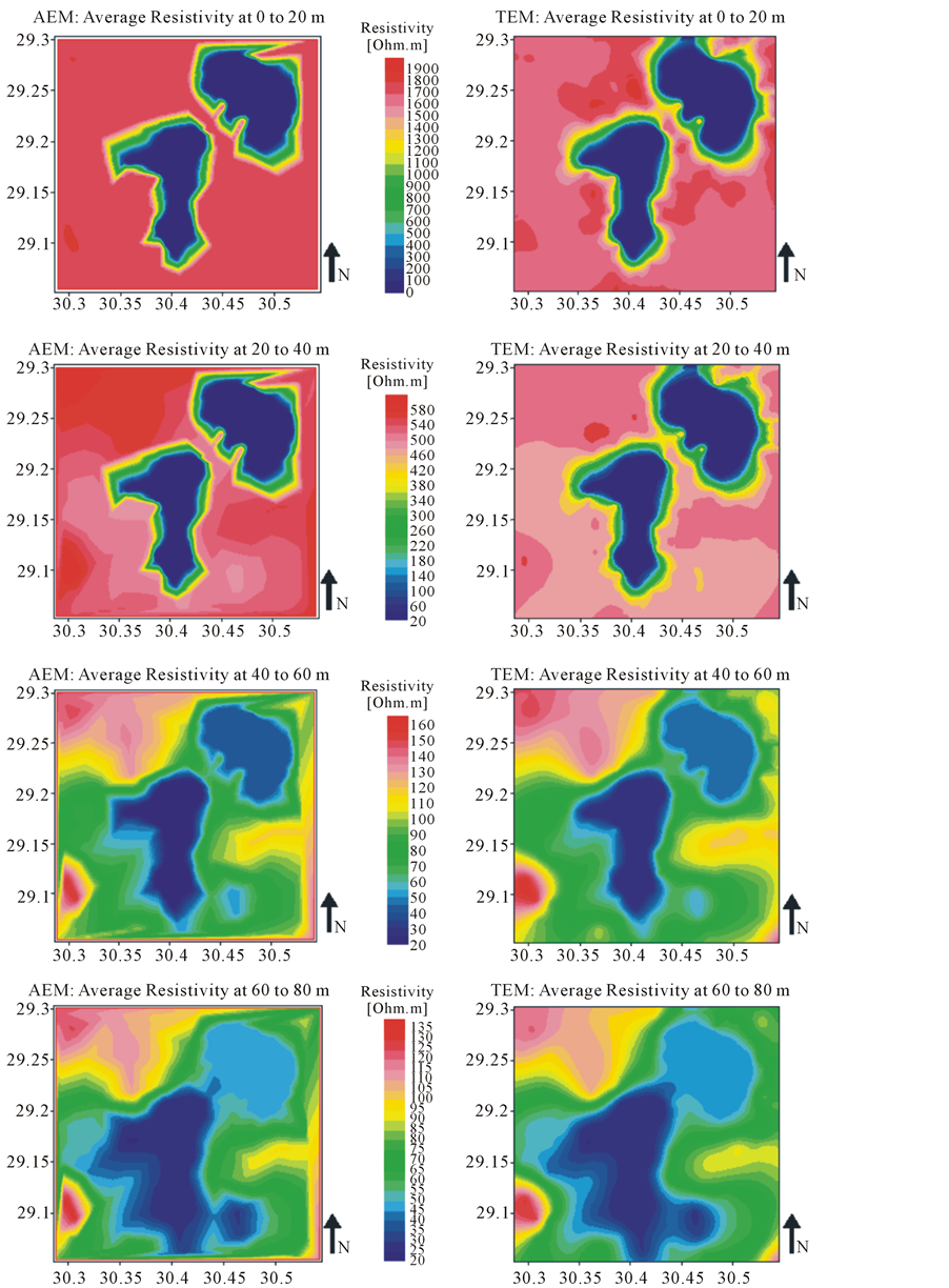
Figure 6. Resistivity maps for different depth ranges derived from 1-D inversion results. On the left hand side the maps of the HEM models and on the right hand side the maps of the TEM models are shown. Two isopach maps from both AEM and TEM method were drowning for the thickness of the fresh water aquifer.
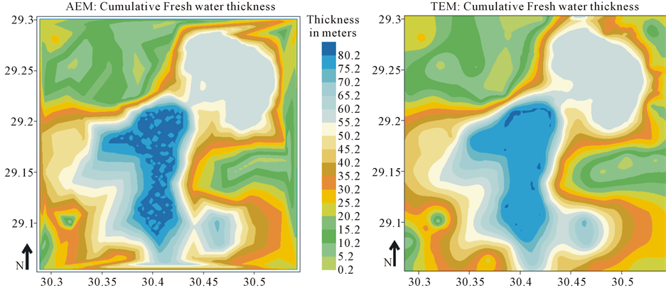
Figure 7. Thickness map of the fresh water derived from HEM (a) and TEM (b) data.
different depth levels. The measured resistivity values have been calculated in an average that accounts every 20 meters from surface to 80 meters in depth. It is clear that the TEM data show more details than AEM.
Two isopach maps from both AEM and TEM method are drawn concerning the thickness of the fresh water aquifer Figure 7. The maps reveal that the thickness of the aquifer ranges from 0 m in some places to 90 m in the middle parts in the basin of lakes.
The resistivity values, from the surface to 20 m depth, range from 1000 Ωm to about 2000 Ωm over the study area. These values may be due to the arid surface layer.
The very low values (less than 100 Ωm) refer to the fresh water in the two lakes in the center and north eastern parts of the area. These low resistivity values are still continuously shown in all maps in the same lake sites. In depth ranges from 20 to 40 m, the resistivity values vary between 220 Ωm and 600 Ωm. This layer may consist of massive gravely sandstone. The maps of depth from 40 to 60 m show resistivity values that range from 20 to 160 Ωm. These maps can witness the first appearance of the fresh water aquifer. The last maps in depth vary from 60 to 80 m, show average resistivity values between 20 and 200 Ωm, these maps may be considered as an extension of the fresh water in the area.
Resistivity models derived from the helicopter borne electromagnetic method are compared with ground time domain electromagnetic method.
Acquired electromagnetic data sets and inversion techniques are applied; the inversion results of both methods are combined in locating the top of a strong conductor (the fresh water) at 56 m depth that has resistivity values between 10 Ωm and 44 Ωm. In this study, AEM is too clear to penetrate fresh water aquifer. It often fails to penetrate it completely. The TEM methods are able to determine the base of the fresh water at more than 80 m depth, but they also fail to reveal the saline water in depth more than 120 m.
HEM and TEM provide detailed information about the resistivity distribution in the near-surface area. They both detect a shallow conductor at 60 m depth (the fresh water). The existence of the fresh water aquifer is confirmed by drilling wells in two sites in the study area.
The investigated depth of the AEM method is limited by the lowest frequency, but with lower frequencies the signal to noise ratio decreases and the weight of the system increases. The lowest AEM frequency that is used is of the order of 100 Hz [23] , i.e. an increase in investigated depth of about 45% compared to that of the BGR system is possible but technically challenging.
References
- Said, R. (1961) Tectonic Framework and Its Influence on Distribution of Forminifera. The American Association of Petroleum Geologists Bulletin, 45, 198-218.
- Tamer, A., El-Shazly, M. and Shata, A. (1975) Geology of the Fayum-Beni Suef Region: Part II Geomorphology. Desert Institute Bulletin, 25, 17-25.
- Tamer, A., El-Shazly, M. and Shata, A. (1975) Geology of the Fayum-Beni Suef Region: Part II Stratigraphy. Desert Institute Bulletin, 25, 27-45.
- Siemon, B. (2009) Levelling of Frequency-Domain Helicopter-Borne Electromagnetic Data. Journal of Applied Geophysics, 67, 206-218. http://dx.doi.org/10.1016/j.jappgeo.2007.11.001
- Palacky, G.J. and West, G.F. (1991) Airborne Electromagnetic Methods. In: Nabighian, M.N., Ed., Electromagnetic Methods in Applied Geophysics, Volume 2 of Investigations in Geophysics No. 3, Society of Exploration Geophysics, Chapter 10, Springer, The Netherlands, 811-879.
- Sengpiel, K.P. and Siemon, B. (1998) Examples of 1D Inversion of Multifrequency AEM Data from 3D Resistivity Distributions. Exploration Geophysics Journal, 29, 133-141. http://dx.doi.org/10.1071/EG998133
- Sengpiel, K.P. and Siemon, B. (2000) Advanced Inversion Methods for Airborne Electromagnetics. Geophysics, 66, 1983-1992. http://dx.doi.org/10.1190/1.1444882
- Nabighian, M.N. (1979) Quasi-Static Response of a Conductive Half-Space. An Approximation Represntstion. Geophysics, 44, 1700-1705. http://dx.doi.org/10.1190/1.1440931
- Hoversten, G.M., Dey, A. and Morrison, H.F. (1982) Comparison of Five Least-Squares Inversion Techniques in Resistivity Sounding. Geophysical Prospecting, 30, 688-734. http://dx.doi.org/10.1111/j.1365-2478.1982.tb01334.x
- Fitterman, D.V. (1986) Transient Electromagnetic Sounding in the Michigan Basin for Groundwater Evaluation: Presented at National Water Assn. Conference-Surface and Borehole Geophysical Methods, Denver, 21 November 1987, 685-692.
- Fitterman, D.V. and Stewart, M.T. (1986) Transient Electromagnetic Sounding for Groundwater. Geophysics, 51, 995-1005. http://dx.doi.org/10.1190/1.1442158
- Valleau, N. (2000) HEM Data Processing—A Practical Overview. Exploration Geophysics, 31, 584-594. http://dx.doi.org/10.1071/EG00584
- Siemon, B., Christiansen, A.V. and Auken, E. (2009) A Review of Helicopter-Borne Electromagnetic Methods for Groundwater Exploration. Near Surface Geophysics, 7, 629-646.
- Beard, L.P. (2000) Comparison of Methods for Estimating Earth Resistivity from Airborne Electromagnetic Measurements. Journal of Applied Geophysics, 45, 239-259. http://dx.doi.org/10.1016/S0926-9851(00)00032-X
- Siemon, B. (2001) Improved and New Resistivity-Depth Profiles for Helicopter Electromagnetic Data. Journal of Applied Geophysics, 38, 65-76. http://dx.doi.org/10.1016/S0926-9851(00)00040-9
- Fraser, D.C. (1978) Resistivity Mapping with an Airborne Multicoil Electromagnetic System. Geophysics, 43, 144-172. http://dx.doi.org/10.1190/1.1440817
- Sengpiel, K.P. (1983) Resistivity/Depth Mapping with Airborne Electromagnetic Survey Data. Geophysics, 48, 181-196. http://dx.doi.org/10.1190/1.1441457
- Sengpiel, K.P. (1990) Theoretical and Practical Aspects of Groundwater Exploration Using Airborne Electromagnetic Techniques. In: Fitterman, D.V., Ed., Developments and Application of Modern Electromagnetic Surveys, US Geolocical Survey Bulletin 1925, Washington DC, 149-154.
- Hodges, G. and Siemon, B. (2008) Comparative Analysis of One-Dimensional Inversions of Helicopter-Borne Frequency-Domain Electromagnetic Data. Proceeding on AEM2008—5th International Conference on Airborne Electromagnetics, Haikko Manor, 28-30 May 2008, 231-239.
- Stephan, Wendland, E. and Fix, G. (1991) Electromagnetic Modeling by Finite Element Methods France Proceeding. Academic Press, London.
- Soliman, M.M.M. (2005) Environmental and Geophysical Assessment of the Ground and Subsurface Water Resources of Ras El-Hekma Area, Northwestern Coast of Egypt. Ph.D., Geophysic, Faculty of Science, Ein Shams University, Cairo.
- TEMIXL XL Program V4 (1996) Temix V.4 User’s Manual, Interpex, 468 p.
NOTES

*Corresponding author.