International Journal of Geosciences
Vol.4 No.1(2013), Article ID:27010,9 pages DOI:10.4236/ijg.2013.41006
An Integrated and Evolutionary Dynamical Systems View of Climate Complexity
Sección de Bioclimatología, Centro de Ciencias de la Atmósfera, UNAM, Circuito Interior s/n, Ciudad Universitaria, Coyoacan, México
Email: walter@atmosfera.unam.mx
Received September 21, 2012; revised November 6, 2012; accepted December 1, 2012
Keywords: Climate Change; Complexity System; Earth
ABSTRACT
The Earth shows a constant display of an organized complexity system, and its intrinsic capacity for sporadic self-organization constitutes its fundamental and profound mysterious property. A graphical method derived from the logistic phase space of precipitation is proposed to identify periods of abundance-scarcity of rain as well as El Niño presence in order to cope with climate change. The most striking result is that the majority of El Niño events on this graph are chaotic, in which the sign of the dominant eigenvalues of precipitation gives trends of scarcity on negative signs and abundance on positive signs, with eleven years periods.
1. Introduction
Simulation of dynamic systems yields conclusions that, among other things help us to make decisions and the outcomes may play another important role in the thinking process and for this purpose, motivation means to interpret and understand the nature of evolution, as well as the emerging weather, ecosystems, life and universe complexity, starting from the point of view of their fundamental simplicity. This principle from dynamics system approach that nature loves simplicity is essential to modern science in order to accept new theories, as much as it is necessary to understand that coevolution is the fundamental movement of the whole universe. From here, we need to adopt a structural perspective that looks into fundamental patterns of climate and life expressions [1-4]. Thus, it is a one-way-search to speak about organisms, ecosystems and climate as a unitary structure, accepting coevolution and seeing the planet as a whole and identifying the climate as a unifying global force, Systems in nature seem disorderly or ruled by random events that seems unpredictable but there is actually hidden order in phase-space rather that in ordinary space and show universality in their approach to chaos like the logistic equation, giving some predictive power [5-10].
Given the close connection between climate and ecosystems, any change in this complexity system is likely to propagate with marked intensity throughout the system with great force, where, small changes in one place may cause chain reactions, nonlinear effects and even environmental disasters. The earth as a homeostatic system is a system that maintains its own state in an ever changing environment by way of internal adjustments. The behavior of the atmospheric system depends on internal and external constraints and its fundamental mechanisms are instability, feedbacks and homeostasis, whose principal manifestations are in their turn bifurcations toward a multiplicity of states [11-16]. Using time delay coordinates we can analyse data on one component of the multidimensional system, without knowing how all the other components behave. A limited cycle in the state space indicates a periodic motion, that is why in systems that have a limit cycle as an attractor, long term predictability is guaranteed. Any random component of exogenous variables is called dynamic noise, which is an integral part of the system’s dynamics affecting how the state variables change over time. The system itself along with external perturbations contribute to the system’s unpredictability.
Equations in a multidimensional system encapsules the endogenous structure of the system or also, its dynamics feedbacks regulating its behavior [17,18]. This means that there are exogenous variables acting on the system as well. But unlike endogenous variables, these are not part of the feedback structure of the system and may have regular, irregular or stochastic patterns of fluctuations, including internal factors of the system which cannot be predicted from state variables.
The most important quantity associated with an exogenous attractor is its dimensionality, which gives us the degree of complexity of the system, though also the number of necessary variables in order to describe the system. What is more important is that it can be used to predict future actions of the system in a long term basis. Such ideas include a geometrical notion of the dimension of correlation as it is used for the mathematical analysis of attractors. Results in the analysis of daily metheorological observations support the existence of those exogenous attractors suggesting that these can be characterized through finite time series of the dynamic systems. Our intention has been to apply these methodologies in matters of short and long term interests, considering the current lack of knowledge about our climate as an exogenous attractor. We believe such methods will allow us not only to develop an understanding of these complex systems, but also to be able to predict their behavior.
2. Methodology
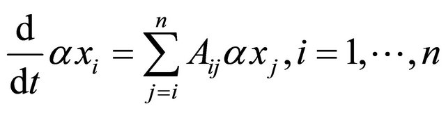
The traditional approach is to solve the nonlineal equations;
 (1)(With n suitable normalized variables xi) twice with slightly different sets of initial conditions. Then the Euclidean norm distance
 , can be evaluated for a sequence of time steps. Beyond the time limit of predictability D (t) would oscillate. If D (t) stays below a value not greater than the difference between two randomly selected states of the system, we can expect predictability for longer time range or to evaluate the growth rates of error dx in the system, which is governed by the set of linear differential Equations (1).
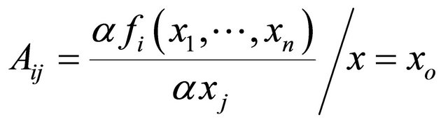
 (2)
(2)
Coefficients Aij are the elements of the Jacobian matrix of f = (fl, ∙∙∙, fn) defined by the partial derivative of (1).
Local stabilities of climate evolution are determined by the eigenvalues, Aij of the Jacobian Matrix which changes with time. The magnitude of the positive characteristic can be used as a measure of unpredictability.
The characteristic exponents refer to the expansion or contration of different directions in the phase space, where the rate of the exponential growth of an infinitesimal vector  in the n-dimensional phase space is given by the largest of the Lyapunov characteristic exponents. Thus the growth rate of the phase space volume element is the growth rate of the Jacobian determinant and it is given by the sum of all n eigenvalues.
We apply the graphic method, Figures 1 and 2 derived from designated properties of the logistic equation for the determination of the corresponding chaotic zone in the space phase in its maximal gradient and for that very reason in its maximun eigenvalue, in the Figures 3-7, Table 1.
Figure 1. Adjustment of precipitation values to logistic equation in order to determine simulation and prognosis coefficients.

Figure 2. Graphic method in order to calculate phase space eigenvalues as well as the system’s behavioural patterns divided in an oscillatory, asymptotic, stable or unstable and chaotic area.

Figure 3. Global temperature anomalies space phases showing in a separate form its multiple attractors and later their integration.
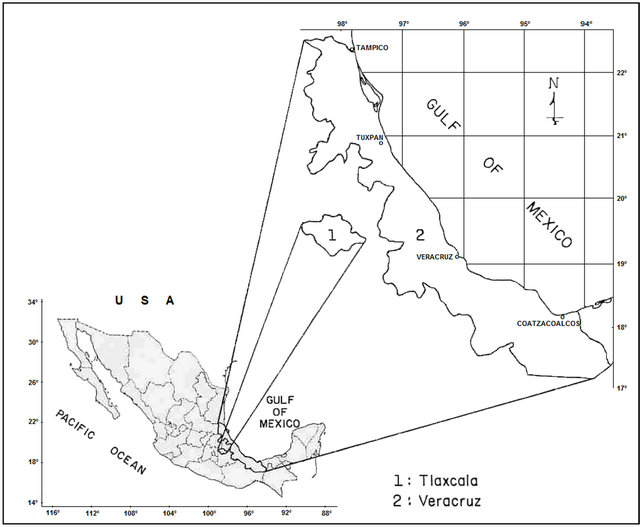
Figure 4. Tlaxcala and Veracruz regions.
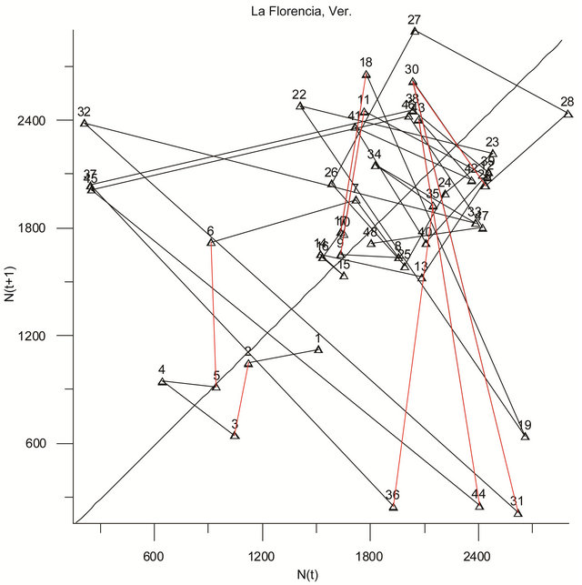

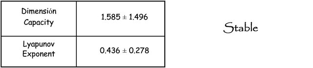
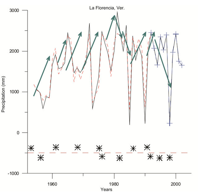
Figure 5. Phase-space of a system with stable/unstable dynamics and corresponding capacity dimension values as well as Lyapunov exponents and autocorrelations, annual precipitation values and their maximum eigenvalues in which positive values correspond to excessive precipitation trends while those negative correspond to deficient trends.
3. Results
Sea surface temperatures exhibited a cooling trend in the Eastern Pacific during the 1980s on about 0.1˚C, followed by a similar warming through 1990, and following closely the 11-year sunspot cycle, where the prime source of global weather comes from the Tropics, in which the weather comes first and later comes El Niño. Apparently ENSO characteristics changed quite markedly over the course of ten years, even in the absence of obvious external forcing.
The accelerated warming that took place in the Central Tropical Pacific during the late twentieth century implies very different forcing and response, in all of the probabilities related to the rise in greenhouse gases. The local stabilities of weather or climate evolution are determined by the eigenvalues or characteristic exponents of the Jacobian matrix where the rate of the exponential growth of an infinitesimal vector in the n-dimensional phase space is given by the largest of the Lyapunov characteristic exponents. The growth rate of the phase space volume elements is the growth rate of the Jacobian determinant and is given by the sum of all the n eigenvalues.
- Precipitation vectors in space phases in the States of Tlaxcala and Veracruz when invading the chaotic area acquire the maximum eigenvalue, which determines the predictive dynamics of the system, Figures 5-7.
- We can observe that through the sign of this eigenvalue we can determine tendencies but also future values in the abundance of regional precipitations. The tendency to positive eigenvalues correspond to abundant rainfall, the tendency to negative eigenvalues to the stablishment of drought situations
- Precipitation vectors in the chaotic area in certain occasions tend to over-stimulate the system, withdrawing from the basic attractor though performing repulsive turns that tend to become predictable with the dynamics of the logistic equation, in its way to chaos, Figures 5 and 6.
- The calculus of precipitation tendencies determined by this methodology in the coastal State of Veracruz and the central State of Tlaxcala, Figure 4, have proved to be correct in over 85% of he total values considered, Figures 5-7.
- Intervals in the forecast of rainfall tendencies start with the critical value of the eigenvalue vector that invades the “chaotic area” and ends up when a new invading vector is introduced in the same area, which will become the new dominant maximum eigenvalue in the dynamics and future tendencies of the system, Figures 5-7.
- Climatological observation stations indicate a higher percentage of unstable tendencies in dry arid regions of both States, while stable tendencies in more productive regions or those with higher levels of precipitation. Such conditions had already been observed, in a comparative rainfall analysis carried out in various areas of the country.
- The presence of El Niño is generally manifested with the appearance of a chaotic behaviour, which can be
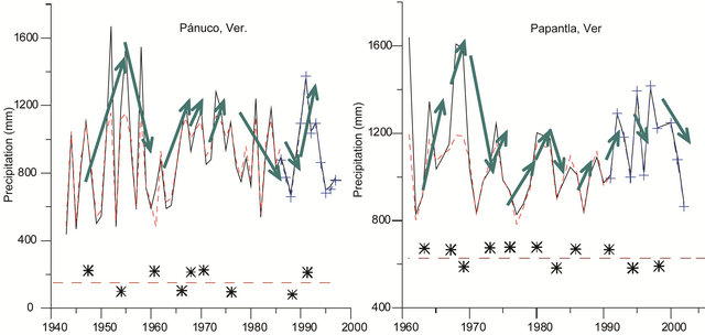
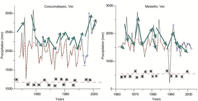

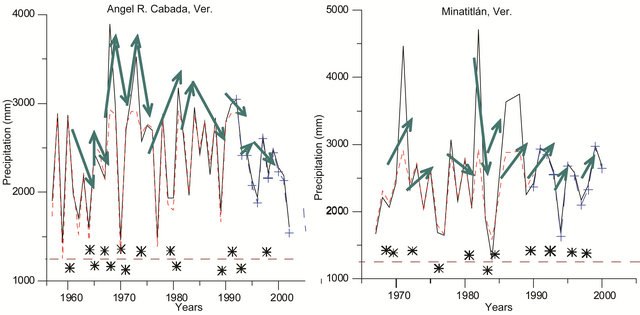
Figure 6. Mean annual precipitation values observed at 6 regions of the Veracruz state and their corresponding prognostic values derived from the logistic equation, in which difference spaces point to those random effects of environmental external noise.

Figure 7. Mean distribution of isohyets (mm/year) for the state of Veracruz for period 1940-2000, and space/dynamic behavior of stable (S)/unstable (U) conditions and significant periodicities (in parenthesis). (NP) means non-significant periods.
Table 1. Global temperatura and tuna Biomass on the Pacific Ocean and El Niño year presence.
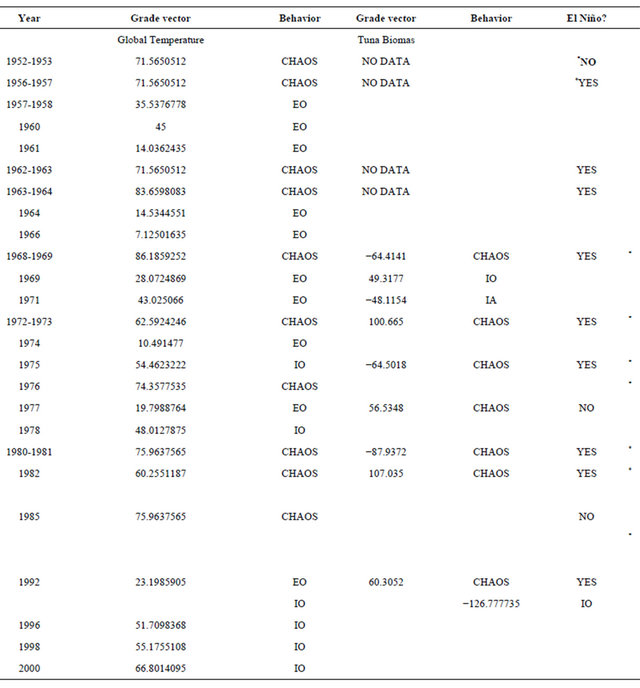
observed in the graphics presented by Figure 2 and Table 1.
- In the stability analysis of ecosystems, we also observe the manifestation of a coevolutive process that corresponds to situations of greater stability when dealing with regions of higher productivity, with 11 years periods, while more instability in drier arid areas and random periods.
- This is detectable in those turns observed in phase spaces that have the greatest percentage of turns directed towards the right in situations of greater stability, and towards the left in unstable situations.
- External factors such as orography (deterministic) along with freezing and northern winds phenomena (stochastic) can actually transform a stable region into an unstable one.
- To apply nonlinear predictive schemata especially in dynamic system models will doubtlessly be a required step to follow in the future to be able to understand as well as to quantify the complexity in the state of weather conditions and climatic systems, including climatic changes.
REFERENCES
- S. Y. Auyang, “Foundations of Complex System Theories in Economics, Evolutionary Biology and Statistical Physics,” Cambridge University Press, Cambridge, 1998.
- S. Ellner and P. Turchin, “Chaos in a Noisy World: New Methods and Evidence from Time-Series Analyses,” The American Naturalist, Vol. 145, No. 3, 1995, pp. 343-375. doi:10.1086/285744
- J. Guckenheimer and P. Holmes, “Nonlinear Oscillations, Dynamical Systems and Bifurcations of Vector Fields,” Springer-Verlag, Berlin, 1983.
- P. Kareva, “Predicting and Producing Chaos,” Nature, Vol. 375, No. 6528, 1995, pp. 189-190. doi:10.1038/375189a0
- T. Y. Lee and Yorke, “Period Three Implies Chaos,” American Mathematical Monthly, Vol. 82, No. 10, 1975, pp. 985-992. doi:10.2307/2318254
- R. M. May, “Biological Populations with Nonoverlapping Generations: Points, Stable Cycles and Chaos,” Science, Vol. 186, No. 4164, 1974, pp. 645-647. doi:10.1126/science.186.4164.645
- R. M. May, “Simple Mathematical Models with Very Complicated Dynamics,” Nature, Vol. 261, No. 5560, 1976, pp. 459-467. doi:10.1038/261459a0
- R. M. May, “Stability and Complexity in Model Ecosystems, Princeton Landmarks in Biology,” Princeton University Press, Princeton, 2001.
- R. M. May and G. F. Oster, “Bifurcations and Dynamic Complexity in Simple Ecological Models,” The American Naturalist, Vol. 110, No. 974, 1976, pp. 573-599. doi:10.1086/283092
- G. Sugihara and R. M. May, “Nonlinear Forecasting as a Way of Distinguishing Chaos from Measurement Error in time Series,” Nature, Vol. 344, No. 6268, 1990, pp. 734- 741. doi:10.1038/344734a0
- R. Pool, “It Is Chaos, or Is It Just Noise?” Science, Vol. 243, 4887, 1989, pp. 25-28. doi:10.1126/science.2911717
- O. W. Ritter, P. A. Mosiño and C. E. Buendía, “Dynamic Rain Model for Lineal Stochastic Environments,” Quaterly Journal of Meteorology, Vol. 49, No. 1, 1998, pp. 127-134.
- O. W. Ritter, O. E. Jauregui, R. S. Guzman, B. A. Estrada, N. H. Muñoz, S. J. Suarez and V. M. C. Corona, “Ecological and Agricultural Productivity Indices and Their Dynamics in a Sub-Humid/Semi-Arid Region from Central México,” Journal of Arid Environments, Vol. 59, No. 4, 2004, pp. 753-769. doi:10.1016/j.jaridenv.2004.02.009
- O. W. Ritter and S. J. Suárez, “Predictability and Phase Space Relationships of Climatic Changes and Tuna Biomass on the Eastern Pacific Ocean,” 6 eme Europeen de Science des Systemes Res-Systemica, No. 5, 2005.
- O. W. Ritter and S. J. Suarez, “Impact of ENSO and the Optimum Use of Yellowfin Tuna in the Easthern Pacific Ocean Region,” Ingenieria de Recursos Naturales y del Ambiente, Cali Colombia, 2011, pp. 109-116.
- S. J. Suarez, W. O. Ritter, C. G. Gay and J. Torres Jacome, “ENSO Tuna-Relations in the Eastern Pacific Ocean and Its Prediction as a Non-Linear Dynamic System,” Atmósfera, Vol. 17, No. 4, 2004, pp. 245-258.
- G. A. F. Seber, “Multivariate Observations,” Jhon Wiley & Sons, New York, 1984. doi:10.1002/9780470316641
- J. H. Vandermeer, “Elementary Mathematical Ecology,” John Wiley, New York, 1972.