Open Journal of Fluid Dynamics
Vol.4 No.1(2014), Article ID:44082,9 pages DOI:10.4236/ojfd.2014.41006
Numerical Analysis of Electromagnetic Control of the Boundary Layer Flow on a Ship Hull
Mohammad Bakhtiari, Hassan Ghassemi
Department of Ocean Engineering, Amirkabir University of Technology, Tehran, Iran
Email: navalarchitect2000@yahoo.com, gasemi@aut.ac.ir
Copyright © 2014 by authors and Scientific Research Publishing Inc.
This work is licensed under the Creative Commons Attribution International License (CC BY).
http://creativecommons.org/licenses/by/4.0/


Received 11 January 2014; revised 11 February 2014; accepted 18 February 2014
ABSTRACT
In this article, electromagnetic control of turbulent boundary layer on a ship hull is numerically investigated. This study is conducted on the geometry of tanker model hull. For this purpose, a combination of electric and magnetic fields is applied to a region of boundary layer on stern so that produce wall parallel Lorentz forces in streamwise direction as body forces in stern flow. The governing equations including RANS equations with SST k-ω turbulent model coupled with electric potential equation are numerically solved by using Ansys Fluent codes. Accuracy of this turbulent model of Fluent in predicting Turbulent flow around a ship is also tested by comparing with available experimental results that it shows a good agreement with experimental data. The results obtained for ship flow show that by applying streamwise Lorentz forces that are large enough, flow is accelerated. The results are caused to delay or avoid the flow separation in stern, increase the propeller inlet velocity, create uniform flow distribution behind the ship’s hull in order to improve the propeller performance, and finally decrease the pressure resistance and total resistance.
Keywords:Electromagnetic Control; Boundary Layer; Turbulent Flow; Flow Separation; Resistance

1. Introduction
The ability to manipulate a flow field to improve efficiency or performance is of immense technological importance. The intent of flow control may be to delay/advance transition, to suppress/enhance turbulence, or to prevent/promote separation. The resulting benefits include drag reduction, lift enhancement, mixing augmentation, heat transfer enhancement, and flow-induced noise. Flow control involves passive or active devices that have a beneficial change on the flow field. During the last decade, emphasis has been on the development of active control methods in which energy, or auxiliary power, is introduced into the flow. One of the active control methods is MHD control. If a fluid is electrically conducting, eelectromagnetic flow control permits to act directly within the boundary layer by applying directly local Lorentz forces.
Mainly three different force configurations have been investigated in order to control turbulent boundary layers: wall parallel streamwise, wall parallel spanwise and nominally wall normal forces. Wall parallel forces in streamwise direction have been applied, e.g., in the experiments of Henoch and Stace [1] and Weier et al. [2] as well as in the numerical analysis of Crawford and Karniadakis [3] . This force configuration increases instead of reducing wall shear stress, because the acceleration of the near wall fluid leads to a higher slope of the mean velocity profile in streamwise direction. However, the momentum gain due to the Lorentz force surpasses the friction drag rise.
Nosenchuck and Brown [4] used nominally wall normal, time dependent forces. Nosenchuck and co-workers reported several successful experiments with a multitude of electromagnetic actuators generating turbulent skin friction reductions.
A circular cylinder equipped with electrodes as well as permanent magnets generating a wall parallel force in streamwise direction was used in the experiments and numerical calculations of Weier et al. [5] . Similar configurations have later been investigated by Kim and Lee [6] , Posdziech und Grundmann [7] , and Chen and Aubry [8] . While skin friction drag is increased by this force configuration, form drag is strongly reduced for an initially separated flow at Reynolds numbers Re = O(100). For stronger forcing, the increase in skin friction drag dominates the form drag decrease. Shatrov and Yakovlev [9] studied numerically the flow around a sphere with a mainly wall parallel Lorentz force at Re up to 1000. For increasing interaction parameter, i.e. the ratio of electromagnetic to inertial forces, the size of the separation region is first reduced. Later, separation is suppressed completely resulting in a strong decrease of form drag. Shatrov and Yakovlev [10] extended the investigated Reynolds number range up to 105 treating the problem of a steady and axially averaged flow. For large Reynolds numbers, the total drag of the sphere was reduced by 4 times and despite the moderate electrical efficiency of  , the total energy consumption was reduced as well.
In present study, electromagnetic control of turbulent boundary layer on a ship hull, without free surface effects, is numerically investigated. For this purpose, a combination of electric and magnetic fields is applied to a region of Turbulent boundary layer on stern so that produce wall parallel Lorentz forces in streamwise direction as body forces in stern flow and their effects on flow parameters such as boundary layer thickness, flow separation, wake distribution on propeller plane, pressure distribution on ship hull and resistance is investigated. This study is done on the geometry of a tanker model hull. Very detailed experimental data are available for this ship [11] . For investigation of Lorentz forces effects, calculations are conducted for two cases without applying electromagnetic field and with applying electromagnetic field locally to stern flow. For this simulation, RANS equations with SST k-ω turbulent model coupled with electric potential equation are used. This governing equation is numerically solved in computational grid generated around ship hull by using Ansys Fluent 14.5 finite volume codes. Accuracy of SST k-ω turbulent model of Fluent in predicting Turbulent flow around a ship is also tested by comparing with available experimental results that it shows a good agreement with experimental data.
2. Governing Equations
2.1. RANS Equations
In this study, it assumed that fluid is incompressible. The governing equations are the mass and momentum conservations. Using the Reynolds averaging approach, the Navier-Stokes equation can be stated as:
 (1)
(1)
 (2)
(2)
where  represents Reynolds stresses and
 is Lorentz body force included in momentom equation for MHD flow
2.2. Turbulent Model
The Reynolds-averaged approach to turbulence modeling requires that the Reynolds stresses in Equation (2) are appropriately modeled. A common method employs the Boussinesq hypothesis to relate the Reynolds stresses to the mean velocity gradients:
 (3)
(3)
In this article, the two-equation Shear-Stress Transport (SST) k-ω turbulence model is used for modeling turbulent viscosity.
The turbulence kinetic energy, k, and the specific dissipation rate, ω, are obtained from the following transport equations:
 (4)
(4)
 (5)
(5)
where  represents the generation of turbulence kinetic energy due to mean velocity gradients:
 (6)
(6)
 represents the generation of ω :
 (7)
(7)
 and
and  are the turbulent Prandtl numbers for k and ω, respectively:
 (8)
(8)
 (9)
(9)
 is cross-diffusion term.
The turbulent viscosity,  , is computed as follows:
 (10)
(10)
where S is the strain rate magnitude, the coefficient  damps the turbulent viscosity causing a low-Reynoldsnumber correction .
 and
and  are blending functions.
2.3. Electric Potential Equation
In general, the electric field  can be expressed as:
 (11)
(11)
where  and
and  are the scalar potential and the vector potential, respectively. For a static field and assuming
  in which
  is induced magnetic field and
  is imposed magnetic field, Ohm's law can be written as:
 (12)
(12)
For sufficiently conducting media, the principle of conservation of electric charge gives:
 (13)
(13)
The electric potential equation is thus given by:
 (14)
(14)
The current density can then be calculated from Equation (12).
With the knowledge of the induced electric current, the MHD coupling is achieved by introducing additional source terms to the fluid momentum equation. This additional source term is the Lorentz force given by:
 (15)
(15)
which has units of  in the SI system.
For MHD flow around a ship hull, the magnetic field induced by the motion of sea water can be neglected compared with the imposed magnetic field. On the other hand, when the electric field is applied, a magnetic field is generated around the electric current. The magnitude of this generated magnetic field is evaluated by integrating Maxwell equation,  , in the region where the electric field is applied:
 (16)
(16)
where I is total electric current and S is area of applied electric field.
 is of
is of  for sea water, and assuming that I is of 103 Amperes at most, this induced magnetic field can again be neglected, in comparison with the imposed magnetic field. So potential electric equation in which the induced magnetic field is neglected, can be a proper method for MHD flow around a ship hull.
Finally, the governing equations to solve become seven equations including four RANS equations, two transport equations for k and ω and one potential equation that must be solved simultaneously.
3. Computational Grid and Boundary Conditions
In present study, a tanker model hull is used for calculate on of flow around ship. This model was presented at CFD workshop in Tokyo [11] . Very detailed experimental data of this ship is available for public use. Main dimensions of this model are shown in Table 1.
Flow around the hull has been considered symmetrical to the center plane of the ship so the calculation is only conducted in on side of the symmetrical plane. Figure 1 shows the computational domain and boundary conditions applied for turbulent flow calculations. The distance of domain boundaries from the ship hull has been considered large enough in order to apply correct boundary conditions. These boundaries include the surface bellow:
1) A spherical surface with a radius of  , that it's center is on the intersection of aft perpendicular and waterplane 2) A cylindrical surface with a radius of
  , that extends for
  from aft perpendicular to downstream flow.
For studying of electromagnetic effects on flow, an external magnetic field is applied to a region of flow limited to following boundaries (by assuming that the origin is on intersection of aft perpendicular and waterplane):
• In longitudinal direction from x = 0.3 m plane to x = 1.3 m plane
• In transverse direction from hull surface to y = 0.5 m plane
• In vertical direction from z = −0.05 m plane to z = 0.25 m plane
Figure 2 represents MHD region and conditions applied to this region. These conditions are:
1) An external magnetic field of  applied in z-axis negative direction.
2) “Conducting Wall” boundary condition with electric potential of  applied on ship hull in MHD region.
Since we have a large change in velocity in the wall normal direction in boundary layer, we need to use

Table 1. Principle dimensions of a tanker model.
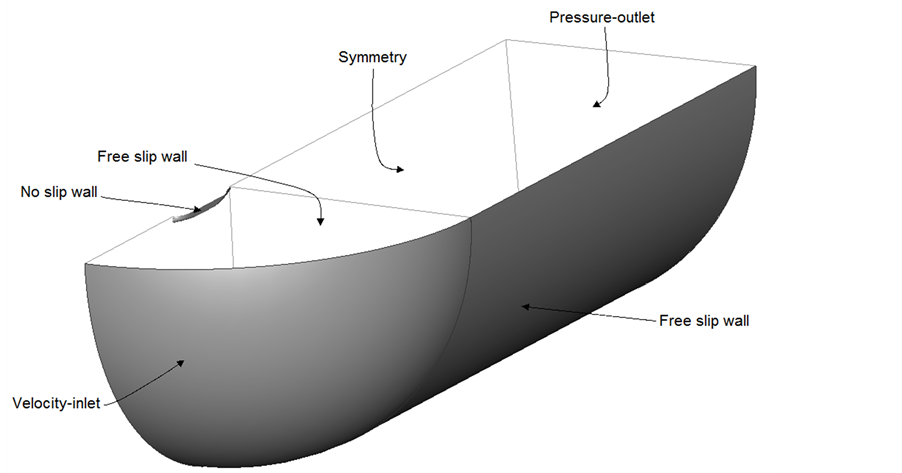
Figure 1. Solution domain and boundary conditions.
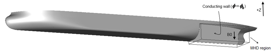
Figure 2. MHD region and conditions applied.
inflation layer meshing with high resolution in boundary layer region. In generating near wall mesh, distance of the first computational node from the wall and numbers of nodes placed within the boundary layer is very important and strongly depends on turbulent model used. We use  as non-dimensional distance of the first node from the wall.
For accurately predicting the velocity profile ,pressure gradients, boundary layer thickness and separation in turbulent boundary layer of ship and also resistance forces (that are of interest in present study), using a low-Reynolds turbulent model to solve whole boundary layer (including laminar sub-layer, Buffer region and fully turbulent layer) is needed. To ensure that we are capturing the laminar sub-layer, the average  value should be on the order of
  and the minimum number of nodes should be between 10 and 20 inside the boundary layer. So in this study, SST k-ω turbulent model is used and the whole solution domain is discretized by structured mesh including hexahedral cells. In order to ensure that the solution is independent of element size and the resolution of generated mesh is fine enough to obtain a numerical solution with minimum discretization error, calculations have been conducted in four computational mesh with different element sizes and cell numbers.
4. Results and Discussions
As mentioned earlier, to investigate the effect of Lorentz forces, two cases were investigated. In the first case, no electromagnetic field was applied, while for the second case, an electromagnetic field was applied locally to stern flow.
We utilized pressure based solver type with Spatial discretization of Body force weighted for pressure and spatial discretization of second order upwind for other field variables.
Calculations are conducted at Froude number  and Reynolds number
  . The working fluid of water has density
 , viscosity
  and electrical conductivity
  .To ensure the convergence of solution , the iterations continues until the residual errors reduce to acceptable value of
  and the total resistance coefficient, Cd, reaches a steady state and in this situation, the imbalance between inlet mass flow rate and outlet mass flow rate is less than 1%.
4.1. Results without MHD
In Table 2, the computed values of resistance coefficients, obtained without free surface effects, are shown. In same table, the total resistance coefficient measured experimentally is also shown. Note a good agreement between the results with a difference of 7%.
A comparison between the computational and experimental results for pressure coefficient distribution on stern is represented in Figures 3. It can be observed that there is a good agreement between computational and experimental results.
Furthermore, the results obtained from numerical computation for axial velocity distribution on the propeller plane compares with experimental results in Figure 4. Again, we can see that computed results show a good agreement with experimental ones.
4.2. Results with MHD
In this section, the computed results with applying electric potential of  volts on ship hull in MHD region as a boundary condition, and an external magnetic field of
  in z-axis negative direction at this region (see figure 2) are represented and then, the effects of Lorentz forces distribution caused by this applied conditions on turbulent boundary layer flow around ship hull is investigated.
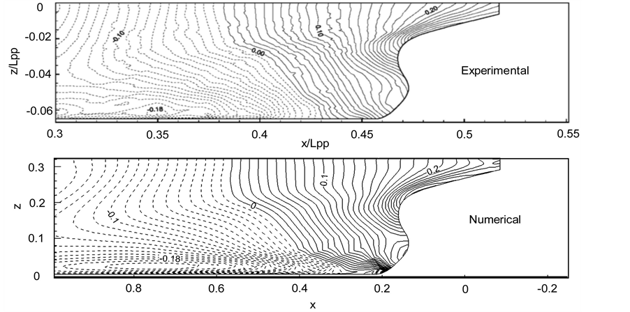
Figure 5 shows the growth of boundary layer flow for two cases (with and without Lorentz forces). The comparison between these two cases demonstrates that the flow is accelerated due to Lorentz forces and boundary layer thickness decreases.
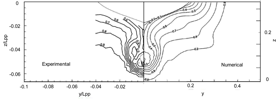
Figure 4. Comparison between experimental and numerical axial velocity distribution on the propeller plane.
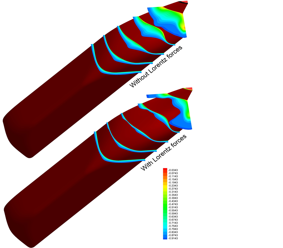
Figure 5. Comparison of boundary layer thickness for two cases (with and without Lorentz forces).
Furthermore, Figure 6 shows a comparison between two cases for axial velocity distributions computed on the propeller plane. From this comparison, it is clear that propeller inlet velocities have increased due to a decrease in boundary layer thickness and separation, which can lead to enhancement in propeller efficiency.
In Table 3, a comparison between computed values of resistances for two cases (with and without Lorentz forces) is shown.
5. Conclusions
In this article, a combination of electric and magnetic fields producing wall parallel Lorentz forces in streamwise direction as body forces, means which were applied to a region of turbulent boundary layer flow on stern of a ship model and its effects on flow around ship hull without free surface effects were numerically investigated. With regard to the numerical results obtained from the calculations, the following conclusions can be offered:
• By applying wall parallel Lorentz forces in streamwise direction to a region of turbulent boundary layer flow on stern of a ship, we can decrease boundary layer thickness and flow separation on stern.
• This type of Lorentz forces can increase axial velocity on propeller plane and so the wake distribution on propeller is improved that leads to enhancement in propeller efficiency.
• The pressure on stern is significantly recovered due to presence of this Lorentz forces, so total ship resistance decreases.
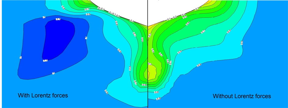
Table 2. Experimental and computational results for resistance coefficients.
Table 3. Computed resistances and their coefficients.
• By using superconducting magnets, we can produce Lorentz forces that are large enough with a much Lower input MHD power. So by lowering the added power due to MHD system, the efficiency of this system can be increased.
References
- Henoch, C. and Stace, J. (1995) Experimental Investigation of a Salt Water Turbulent Boundary Layer Modified by an Applied Streamwise Magnetohydrodynamic Body Force. Physics of Fluids, 7, 1371-1383. http://dx.doi.org/10.1063/1.868525
- Weier, T., Fey, U., Gerbeth, G., Mutschke, G., Lielausis, O. and Platacis, E. (2001) Boundary Layer Control by Means of Wall Parallel Lorentz Forces. Magnetohydrodynamics, 37, 177-186.
- Crawford, C.H. and Karniadakis, G.E. (1997) Reynolds Stress Analysis of EMHD-Controlled Wall Turbulence: Part I Streamwise Forcing. Physics of Fluids, 9, 788-806. http://dx.doi.org/10.1063/1.869210
- Nosenchuck, D. and Brown, G. (1993) Discrete Spatial Control of Wall Shear Stress in a Turbulent Boundary Layer. In: So, R., Speziale, C. and Launder, B., Eds., Near-Wall Turbulent Flows, Elsevier, Amsterdam.
- Weier, T., Gerbeth, G., Mutschke, G., Platacis, E. and Lielausis, O. (1998) Experiments on Cylinder Wake Stabilization in an Electrolyte Solution by Means of Electromagnetic Forces Localized on the Cylinder Surface. Experimental Thermal and Fluid Science, 16, 84-91. http://dx.doi.org/10.1016/S0894-1777(97)10008-5
- Kim, S. and Lee, C. (2000) Investigation of the Flow around a Circular Cylinder under the Influence of an Electromagnetic Force. Experiments in Fluids, 28, 252-260. http://dx.doi.org/10.1007/s003480050385
- Posdziech, O. and Grundmann R. (2001) Electromagnetic Control of Seawater Flow around Circular Cylinders. European Journal of Mechanics, 20, 255-274. http://dx.doi.org/10.1016/S0997-7546(00)01111-0
- Chen, Z. and Aubry, N. (2005) Active Control of Cylinder Wake. Communications in Nonlinear Science and Numerical Simulation, 10, 205-216. http://dx.doi.org/10.1016/S1007-5704(03)00128-X
- Shatrov, V. and Yakovlev, V. (1985) Hydrodynamic Drag of a Ball Containing Aconduction-Type Source of Electromagnetic Fields. Journal of Applied Mechanics and Technical Physics, 26, 19-24. http://dx.doi.org/10.1007/BF00919618
- Shatrov, V. and Yakovlev, V. (1990) The Possibility of Reducing Hydrodynamic Resistance through Magnetohydrodynamic Streaming of a Sphere. Magnetohydrodynamics, 26, 114-119.
- Hino, T. (2005) CFD Workshop Tokyo 2005. National Maritime Research Institute, Tokyo.