Journal of Applied Mathematics and Physics
Vol.04 No.07(2016), Article ID:68163,9 pages
10.4236/jamp.2016.47127
Maximum Entropy and Bayesian Inference for the Monty Hall Problem
Jennifer L. Wang1, Tina Tran1, Fisseha Abebe2
1Norcross High School, Norcross, GA, USA
2Department of Mathematics and Statistics, Clark Atlanta University, Atlanta, GA, USA

Copyright © 2016 by authors and Scientific Research Publishing Inc.
This work is licensed under the Creative Commons Attribution International License (CC BY).
http://creativecommons.org/licenses/by/4.0/


Received 15 May 2016; accepted 8 July 2016; published 11 July 2016
ABSTRACT
We devise an approach to Bayesian statistics and their applications in the analysis of the Monty Hall problem. We combine knowledge gained through applications of the Maximum Entropy Principle and Nash equilibrium strategies to provide results concerning the use of Bayesian approaches unique to the Monty Hall problem. We use a model to describe Monty’s decision process and clarify that Bayesian inference results in an “irrelevant, therefore invariant” hypothesis. We discuss the advantages of Bayesian inference over the frequentist inference in tackling the uneven prior probability Monty Hall variant. We demonstrate that the use of Bayesian statistics conforms to the Maximum Entropy Principle in information theory and Bayesian approach successfully resolves dilemmas in the uneven probability Monty Hall variant. Our findings have applications in the decision making, information theory, bioinformatics, quantum game theory and beyond.
Keywords:
The Monty Hall Problem, Conditional Probability, Nash Equilibrium, Bayesian Inference, Maximum Entropy Principle

1. Introduction
The famous Monty Hall problem arises from a popular television game show Let’s Make a Deal [1] [2] . In the game, a contestant faces three closed doors. One of the closed doors conceals a brand new car, whereas the other two doors conceal goats that are worthless. To start with, the show host, Monty, asks the contestant to choose a door as the initial guess. After the contestant chooses a door, Monty opens another door that conceals a goat. Then, Monty offers the contestant the option to stick with the door selected initially, or switch to the other closed door. An interesting question arises as to what are the advantages and disadvantages of frequentist and Bayesian statistical techniques in incomplete information games such as the Monty Hall problem, and what is the potential impact of these approaches on decision-making in a variety of scientific areas.
As a mathematical problem, it is important to clarify the rules of the game that are not necessarily in parallel to the realistic game show situations. For the Monty Hall problem, Monty is required to open a goat-yielding door not chosen by the contestant under all circumstances [1] - [3] . As such, even though the winning opportunity appears to be 50:50 for the two remaining doors, the counter-intuitive answer is that the contestant should switch. The update of probability, conditional upon the constraint that Monty cannot open the door selected by the contestant, is pivotal to recognize the difference between the two closed doors [2] . When the contestant selects a
door, there is a  chance of being right and a
  chance of being wrong. After Monty opens a goat-yielding door, the door initially held by the contestant remains the same
  winning probability, whereas the other closed door now has a
  winning chance. Therefore, the contestant should switch to maximize the chance of winning
the prize. In general, Bayesian inference indicates that the constraint as mentioned above leads to dividing the probability space into two sets. One set contains the door initially chosen by the contestant with prior probability , and the other set contains the other doors with probability
 . In the end, the decision depends merely on the comparison of
  and
and  since the goat-yielding actions are not supposed to change
 . However, this conceivably simple Bayesian reasoning for the Monty Hall problem has been the subject of open debate [1] .
The controversy focuses on the correct way of updating information between Bayesian and frequentist appro- aches to statistics [1] . Bayesian inference’s assertion that the probability of the initially chosen door remains intact after Monty’s goat-yielding action is precisely the point at issue. In fact, the frequentist approach indicates that the probability  may change [1] . The frequentist inference entails that Monty makes his choice at random when given a selection of doors to open [1] - [9] . Frequentist and Bayesian inferences result in different answers for variants of the problem. For example, what if the prior probability of placing the car behind each door is not equal? What if, given a choice, Monty prefers to open one door over another? Given that the frequentist approach is used exclusively in the literature [1] - [11] , it becomes necessary to develop Bayesian approaches for the Monty Hall problem.
In this paper, we discuss and analyze a few variations of the Monty Hall problem to clarify the difference between Bayesian and frequentist inferences. We model the problem as an incomplete information game in which Monty and the contestant have opposing interests [10] - [12] . The solution of the Monty Hall game involves the determination of Nash equilibrium strategies, one for the contestant and the other for Monty [13] . We employ the Maximum Entropy Principle [14] to devise the optimal strategy for Monty, which corresponds to an “irrelevant, therefore invariant” theorem [1] [13] . In contrast, the “coin-flipping” procedure [1] [2] is shown to be unjustified for an uneven variant of the Monty Hall problem. Our findings not only completely resolve the Monty Hall problem and its variants, but also have applications in the decision making, information theory [14] , bioinformatics [15] - [17] , quantum game theory [11] [12] and beyond.
2. Methods
2.1. Bayes’ Theorem
Bayes theorem serves as an approach to statistical inference by means of conditional probabilities. Bayes theo- rem states that for two events C and O, the probability of C given O,  , is related to the likelihood of O given C,
  , as:
, as:
 (1)
(1)
We define , and
, and  to be the events in which the car is placed behind door A, B, and C, respectively [1] . Let’s assume that the contestant selects door A. Since Monty cannot open either door A (the contestants initial choice) or the door with the car, we have
 , where
 , and
, and  denote the events in which Monty opens door A, B, or C to reveal a goat, respectively.
If the contestant’s initial choice is wrong (i.e., the car is not behind door A), Monty’s option to open a door is restricted in that if the car is behind B or C, then the host has to open door C or B, respectively. We have
 . On the other hand, if the contestant’s initial choice is correct (i.e.,
 ), the host can freely choose between one of the two doors, B or C. We can treat the parameter
  (we have
 ) as a random variable ranging from 0 to 1, reflecting the likelihood that Monty exhibits a bias in favor of selecting door B (or C) if the car is behind door A.
Given that the possibility of finding the car behind door A, B, or C is equally likely, and then we have
 . We evaluate the probability for Monty to open door B using the law of total proba-
bility,
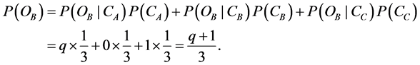 (2)
(2)
Substituting everything into Bayes theorem, we obtain
 (3)
(3)
Similarly for Monty opening door C, we have
 (4)
(4)
 (5)
(5)
The frequentist inference estimates Monty’s decision procedure q by means of long-run successful frequencies [5] - [9] , and subsequently determines whether to stick or switch by evaluating
 or
or . As seen from Equation (3) and Equation (5), one can infer that switching is optimal for the contestant in that
  for
for , and
, and
 for
for .
.
Bayesian inference uses expected values to determine the optimal option:
 (6)
(6)
 (7)
(7)
Calculated expected values for sticking and switching are independent of q; thereby supporting the argument that rational decision in the single case is not relevant to the degrees of belief about long-run success frequency [4] - [9] . For a single game, Monty’s goat-yielding action is realized by selecting a discrete value of  or 0. The frequentist approach typically uses a “coin-flipping” procedure for the bias parameter q. On the other hand, the expected value includes contributions from
  and
and , irrespective of in reality
  or
or . In other words, Bayesian inference takes into account not only what happened but also what could happen.
If  and
and , then frequentist and Ba- yesian approaches lead to the same result. However, if e.g.,
  , then two approaches yield different answers. To have an in-depth understanding of the differences between frequentist and Bayesian in- ferences, we employ tools in information theory to calculate the conditional entropy.
2.2. Conditional Entropy
In information theory, Shannon entropy is the average amount of information contained in each event. If  or
or  is the probability of the event
  or
or ,
,  , or C, then its entropy is
 . Shannon entropy also measures uncertainty about an event. The less likely an event is, the more information it provides when the event occurs, and vice-versa. The combined system OC is characterized by a joint probability
  and therefore by a joint entropy
 , which is the uncertainty about the entire system. The conditional entropy is defined as
 (8)
(8)
where  is the probability of
  conditional on
 ;
;  characterizes the remaining uncer- tainty about the event C when O is known.
In the literature of discussing the Monty Hall problem, few have brought up the concept of conditional entropy. We utilize the Maximum Entropy Principle [14] to infer rational decision by Monty from the information theory perspective. The Maximum Entropy Principle [14] refers to finding the distribution that represents the highest uncertainty. In the Monty Hall problem, the principle resembles the premise that Monty can follow a strategy to provide the contestant with minimal information. The use of Maximum Entropy Principle reproduces every aspect of Bayesian inference and demonstrates the compatibility of Bayesian and entropy methods.
2.3. Nash Equilibrium
What is the rational response in the case where the host adopts a strategy that minimizes the winning chance of the contestant [11] - [13] ? To answer this question, we need to consider the connection between the strategies chosen by both the host and the contestant. In the Monty Hall problem, Monty’s decision procedure is characte- rized by a bias parameter q, and the contestant’s decision process is described by a parameter p, which is the probability of sticking. The Nash equilibrium recognizes those combinations of strategies for the contestant and host in which each is making the optimal choice given the choice that the other makes. A Nash equilibrium study allows for a thorough evaluation of not only optimal strategies but also sub-optimal strategies. Nash equilibrium strategies are self-enforcing because either player will be worse off if they deviate from the Nash equilibrium. Our analysis of Nash equilibrium strategies prevails in resolving the controversy over dilemmas appearing in the variants of the Monty Hall problem.
3. Results and Discussion
Preceding investigations [1] - [11] into the Monty Hall problem focused predominantly on the winning chances of sticking and switching, which arises from differences between free choice (unconditional probability) and restricted choice (conditional probability). Depicted in Figure 1 are results from the so-called free choice and restricted choice scenarios. The free choice refers to the case where Monty may open a goat-yielding door even if it is selected by the contestant [1] - [3] . It is then easy to show that the winning chance for sticking or switching strategies becomes 50:50. In contrast, with restricted choice, the winning chance for sticking and switching is
 and
and , respectively [1] .
The “coin-flipping” has been used exclusively in the literature [1] - [11] . The coin-flipping entails that Monty chooses randomly from his options when door A conceals the car , which amounts to
 . In other words, Monty may open either B or C, and the approximation requires him to show no preference
to either door. With the use of the “coin-flipping”, the subsequent probabilities can be extracted from Equation
(3) or Equation (5). In either case ( or
or ), the winning probability of sticking is
 , and that of switching is
  [1] .
[1] .
Figure 2 displays the calculated conditional entropy as a function of the bias parameter,
 (9)
(9)
As seen in Figure 2, the maximum entropy of the symmetrical curve is at , whereas the minimum en-
tropy endpoints are at  or
or . In the absence of information about the selection process used by Monty, expected values of winning the prize for sticking or switching are independent of the process (see Equation (6) and Equation (7)), which coincide with the assessed likelihood using the frequentist approach with
 . Suppose that Monty chooses
  (or
(or ) and informs the contestant accordingly before the game
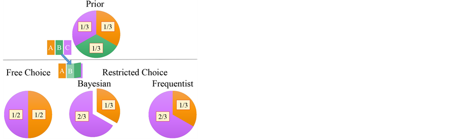
Figure 1. The probability distribution of prior (top panel), free-choice (bottom left), restricted choice with Bayesian inference, and restricted choice with frequentist approach (bottom right).

Figure 2. Calculated Shannon entropy as a function of the parameter q for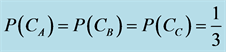 . Insets: the winning probability of the contestant initially selecting the green door and Monty opening either the light or dark grey door, respectively.
starts, we have a strongly biased scenario as a variant of the original Monty Hall problem [6] . In this situation,
there is a  chance that the contestant knows exactly the location of the car if Monty opens the non-preferred
door. In the case that Monty opens the preferred door, the contestant has a 50:50 winning chance for either sticking or switching. It is important to note that there is a difference between the case where Monty informs the contestant of his decision process before a door is chosen and the case in which he informs the contestant after. In the latter case, Monty has gained additional information, which is not accounted for by frequentist inferences.
The frequentist approach entails using a fixed model to the inference [1] . Consequently, the “coin-flipping”
assumption ( ) has been used exclusively in the literature for the solution of variants of the Monty Hall
problem [1] - [11] . However, Monty is not compelled to “coin-flipping”. In reality, Monty should adopt strategies to reduce the contestants winning chance. For Bayesian inference, although the partition of the probability space argument has been elaborated on before, there is a striking lack of analysis on its underlying ramifications. Converting Bayesian inference (the probability of that initially selected door concealing the car is invariant of the event of Monty opening a goat-yielding door) into conditional probability formalism, we have:
 (10)
(10)
This indicates that the events of  and
and  are independent; so are
  and
and . This independence also implies that
 .
.
Using the law of total probability, we can calculate the bias parameter q:
 (11)
(11)


There exists a bias parameter q that characterizes the result of Bayesian inference, which facilitates an assess- ment of epistemic and statistical probabilities for Bayesian and frequentist inferences [4] - [9] .
A few remarks are immediately in order. 1) As a conditional probability problem, it is important to remove ambiguities through the rules of the game [1] - [3] . The following rules are necessary: Monty by no means opens the goat-yielding door the contestant chose initially, and Monty always opens a door concealing a goat [1] [2] . The former is essential for the partition of the probability space. The latter is important as well in case Monty
limit the winning chance of the contestant to  by ending the game prematurely [10] ; 2) If the contestant initially
chooses the correct door, Monty then faces with a choice as to which door to open. The frequentist approach uses a “coin-flipping” method [1] . In Bayesian approach, however, Monty can choose to open a door in such a way that no additional relevant information is given to the contestant; 3) For the two non-selected doors with the same prior winning probability, the two approaches find the same solution. However, the reasoning behind each
answer varies. In the frequentist inference, q is assumed to be  [1] , whereas Bayesian inference determines the value of q to be
 . When the non-selected doors have different prior winning probabilities, the frequentist and
Bayesian inferences lead to different results.
To illustrate the differences, we examine an uneven probability model in which the odds of a car being behind a door are not uniform. A case of an unequal prior model could occur as follows. Assume Monty rolls a standard, 6-sided die. If he rolls a 1, 2, or 3, then the car is placed behind door A. If he rolls a 4 or 5, the car is placed behind door B. If he rolls a 6, the car is placed behind door C. Therefore, the winning probabilities for the doors
 , and C, are
 ,
,  , and
, and , respectively. The contestant consequently rolls the die to select a door as the
contestant’s initial choice.
Shown in Figure 3 are the results that the contestant initially chooses door A. According to the “coin-flipping”,
for ,
,  and
and  [1] . Therefore, it is in the contestant’s best interest to stick. Conversely, for
 ,
,  and
and . Then the contestant should switch in this case [1] .
Monty, however, has a counter strategy available. If , Monty opens door C (
 ), the contestant switches doors and loses. If
 , on the other hand, Monty opens door B (
 ), the contestant sticks to the initial choice and also loses. The only case in which the contestant wins is
 , in which case Monty has to open door C (
 ),
),
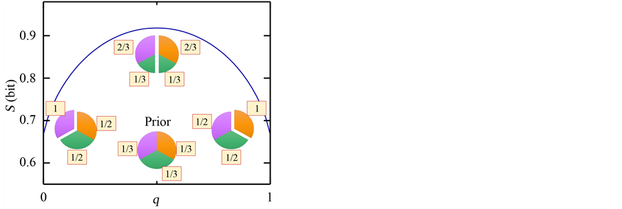
Figure 3. Probability distribution changes from the prior to the restricted choice with the frequentist inference (left panel) and to that with Bayesian inference (right panel), respectively.
the contestant switches to door B and wins. This counter-strategy limits the contestant’s winning chance to , instead of
  for a mixed strategy by randomly sticking or switching with equal probability.
In fact, the case where  allows for a straightforward evaluation of the Nash equilibrium strategy. We have
 (12)
(12)
 (13)
(13)
As a consequence, if , the contestant should switch for
  and stick for
 ; whereas if
 , the contestant should stick for
  and switch for
 . Consequently, Monty’s dominant strategy is for bias parameter
 . At
. At ,
,  ,
,  ,
,
where  and
and  are calculated expected values following Equation (6) and Equation (7). It is straightforward to evaluate the tactics of the contestant and conclude that the contestant should then decide ran-
domly between switching and sticking, i.e., .
.
It is worth noting that the Nash equilibrium is at ( ). The result of
  is a stark contrast to the “coin-flipping” that assumes
 . Therefore, an extension of the “coin-flipping” to variants of the Monty
Hall problem is unjustified. In contrast, using Bayesian inference (cf. the derivations of Equation (11)), we have
 (14)
(14)
Therefore, the rational decision procedure inferred from Bayesian approach conforms to the Nash equilibrium
strategy. Furthermore, we have  and
and
 for Bayesian inference.
To further pursue this point, we calculate the conditional entropy as the function of the bias parameter (q) for the initial unequal probability model,
 (15)
(15)
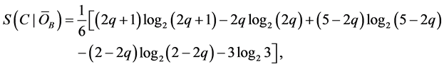 (16)
(16)
 (17)
(17)
where , and
, and  represents
 , and
, and , respectively.
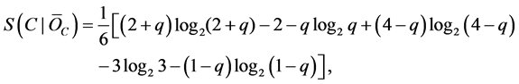
As seen in Figure 4, the maximum entropy for each instance is , and
, and  for
for , and
, and , re-
, re-
spectively. It is worth noting that Bayesian approach yields the maximum entropy value of q, which corresponds to the rational strategy for Monty. We summarize in Table 1 extracted values of conditional entropy for different
bias parameters. The value of  is larger than the corresponding value of the “coin-flipping”
  for the
uneven probability model.
We have demonstrated that Bayesian inference corresponds to Maximum Entropy solution for the calculated conditional entropy. As a result, Bayesian approach can be employed to tackle the variants of the Monty Hall problem. In contrast, if the contestant miscalculates rational decisions by the “coin-flipping” model, we have demonstrated that there exists a counter strategy for Monty to take advantage of the situation.
4. Conclusions
In conclusion, we have devised a Bayesian inference approach for a systematic exploration of rational decisions for variants of the Monty Hall problem. The method employs the Maximum Entropy Principle [14] . Our results show that the “coin-flipping” assumption is unfounded in several variants of the Monty Hall problem. In contrast, Bayesian inference considers many different perspectives in updating the probability to avoid inference bias.
The frequentist inference determines the winning probability using single conditional probability. Bayesian inference estimates the winning probability using expected values that are weighted averages of individual conditional probabilities. Bayesian inference considers Monty’s decision process with respect to the change of information at the various stages of the game. We examined a few variants of the Monty Hall problem and showed that the “coin-flipping” assumption was in general not consistent with maximum entropy solutions. Our analysis on the uneven prior probability Monty Hall variant reveals fallacies in the “coin-flipping” assumption, thereby providing convincing evidence that Bayesian inference is appropriate in tackling Monty Hall-like conditional
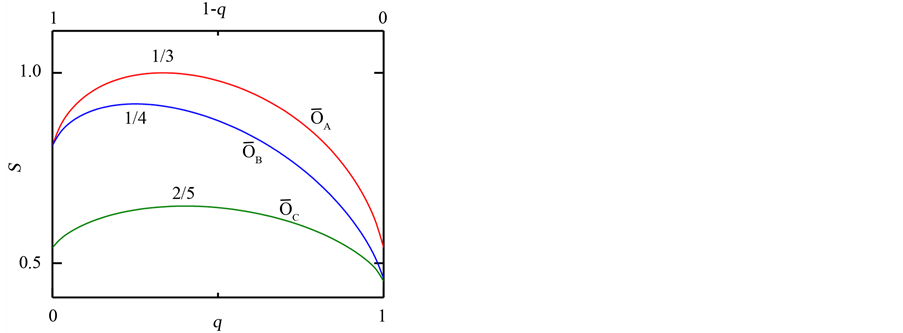
Figure 4. Calculated Shannon entropy for the unequal prior probability model , and
, and .
.

Table 1. Extracted Shannon entropy S for the original model, and  for the unequal probability model
 ,
,  , and
, and  as a function of the bias parameter q.
probability problems. We believe that our findings shed light on the application of Bayesian inferences and the Maximum Entropy Principle in quantum Monty Hall problems [11] [12] , which deserve further development in the future.
We remark, before closing, that the approaches developed in this paper can be applied to a variety of emerging fields, notably Big Data and Bioinformatics. Bayesian inference has some appealing features, including the capa- bility of describing complex data structures, characterizing uncertainty, and providing comprehensive estimates of parameter values, and comparative assessments. Bayesian methodology can be employed for a comprehensible means of integrating all available sources of information and of considering missing data. There is also of great benefit in using Bayesian approach as a mechanism for integrating mathematical models and advanced compu- tational algorithms.
Acknowledgements
The idea of the present research came up in discussions during a Math Team lecture regarding the Monty Hall problem and the Prisoner’s Dilemma. We are grateful for fruitful discussions with Professors P. Baumann, W. Mao, J. Rosenhouse, W. Seffens, and X. Q. Wang. The work at Clark Atlanta University was supported in part by the National Science Foundation under Grant No. DMR-0934142.
Cite this paper
Jennifer L. Wang,Tina Tran,Fisseha Abebe, (2016) Maximum Entropy and Bayesian Inference for the Monty Hall Problem. Journal of Applied Mathematics and Physics,04,1222-1230. doi: 10.4236/jamp.2016.47127
References
- 1. Rosenhouse, J. (2009) The Monty Hall Problem. Oxford University Press, New York.
- 2. vos Savant, M. (1991) Marilyn vos Savant’s Reply. The American Statistician, 45, 347-348.
- 3. Gardner, M. (1959) Problems Involving Questions of Probability and Ambiguity. Scientific American, 201, 174-182.
http://dx.doi.org/10.1038/scientificamerican1059-174 - 4. Baumann, P. (2005) Three Doors, Two Players, and Single-Case Probabilities. American Philosophical Quarterly, 42, 71-79.
- 5. Baumann, P. (2008) Single-Case Probabilities and the Case of Monty Hall: Levy’s View. Synthese, 162, 265-273.
http://dx.doi.org/10.1007/s11229-007-9185-6 - 6. Rosenthal, J.S. (2008) Monty Hall, Monty Fall, Monty Crawl. Math Horizons, 16, 5-7.
- 7. Levy, K. (2007) Baumann on the Monty Hall Problem and Single-Case Probabilities. Synthese, 158, 139.
http://dx.doi.org/10.1007/s11229-006-9065-5 - 8. Tubau, E., Aguilar-Lleyda, D. and Johnson, E.D. (2015) Reasoning and Choice in the Monty Hall Dilemma: Implications for Improving Bayesian Reasoning. Frontiers in Psychology, 6, 353.
http://dx.doi.org/10.3389/fpsyg.2015.00353 - 9. Sprenger, J. (2010) Probability, Rational Single-Case Decisions, and the Monty Hall Problem. Synthese, 174, 331-340.
http://dx.doi.org/10.1007/s11229-008-9455-y - 10. Schuller, J.C. (2012) The Malicious Host: A Minimax Solution of the Monty Hall Problem. Journal of Applied Statistics, 39, 215.
http://dx.doi.org/10.1080/02664763.2011.580337 - 11. Flitney, A.P. and Abbott, S. (2002) Quantum Version of the Monty Hall Problem. Physical Review A, 65, Article ID: 062318.
http://dx.doi.org/10.1103/PhysRevA.65.062318 - 12. D’Ariano, G.M., et al. (2002) The Quantum Monty Hall Problem. Quantum Information and Computation, 2, 355.
- 13. Pawlowski, M., et al. (2009) Information Causality as a Physical Principle. Nature, 461, 1101-1104.
http://dx.doi.org/10.1038/nature08400 - 14. Jaynes, E.T. (1988) The Relation of Bayesian and Maximum Entropy Methods. In: Erickson, G.J. and Smith, C.R., Eds., Maximum-Entropy and Bayesian Methods in Science and Engineering, Vol. 31-32, Springer, Netherlands, 25-29.
http://dx.doi.org/10.1007/978-94-009-3049-0_2 - 15. Eddy, S.R. (2004) What Is Bayesian Statistics? Nature Biotechnology, 22, 1177-1178.
http://dx.doi.org/10.1038/nbt0904-1177 - 16. Stephens, M. and Balding, D.J. (2009) Bayesian Statistical Methods for Genetic Association Studies. Nature Reviews Genetics, 10, 681-690.
http://dx.doi.org/10.1038/nrg2615 - 17. Pharchenko, P.V., Silberstein, L. and Scadden, D.T. (2014) Bayesian Approach to Single-Cell Differential Expression Analysis. Nature Methods, 11, 740-742.