Theoretical Economics Letters
Vol.4 No.7(2014), Article ID:48481,10 pages
DOI:10.4236/tel.2014.47069
An Alternative View to the Cause of Market Failures: A Dynamic Approach
Salvador Contreras
University of Texas Pan American, Edinburg, USA
Email: contrerass@utpa.edu
Copyright © 2014 by author and Scientific Research Publishing Inc.
This work is licensed under the Creative Commons Attribution International License (CC BY).
http://creativecommons.org/licenses/by/4.0/


Received 31 May 2014; revised 30 June 2014; accepted 28 July 2014
ABSTRACT
This paper presents an alternative view to the cause and size of market failures. The work here suggest that the size of the market failure is not man made per se but rather given a full set of initial conditions it is endogenous to the dynamical forces at play. It is shown that the level and variance of market failures is tied to the location of the steady state (i.e. level of development). The paper finds that only changes to the location of the steady state produces changes to the potential level of the market failure. This paper adds to the increasing body of literature the notion that institutional change is not a sufficient condition to sustained economic development.
Keywords:Market Failure, Corruption, Institutional Change, Development

1. Introduction
Corruption and corruption abatement are an important string in economic theory because corruption is seen as a major source of economic instability and a leading cause of poverty among the worlds poor countries ([1] -[3] ). The literature claims that the market failure to properly clear is one of the primary drivers of corruption. [4] begin their exercise by proposing that government intervention, and with it the rise of corruption, is driven by a desire to correct market failures. This strand of the literature has developed models where public agents (bureaucrats) use their positions to extract payments (for personal gain) from private agents ([4] -[6] ). In doing so, [4] show that a positive level of corruption may be socially acceptable since the eradication of corruption is costlier than the negative effect of the market failures it is trying to correct.
The empirical literature on corruption has shown that there exist positive levels of some form of corruption in both rich and poor countries alike ([7] ). [1] further ties growth to perception of corruption1. The evidence show that poorer countries suffer from higher levels of corruption ([1] [3] [7] ). That is, tying corruption to market failures, poorer countries are more likely to face market failures and hence greater incidence of government intervention and with it increase likelihood of bureaucratic corruption.
The economic policy is to reform the institutions that allow for information asymmetries and weak legal enforcement environments to exist as a means of tackling market failures. However, [9] has shown that a large number of standard issue economic fixes are not effective at combating the illness that affect most poor countries. It is this paradox that this paper aims to address. This paper builds a theoretical model that produces an endogenous level of the size of the market failure. However, this paper takes a different view as to how market failures arise. The approach here is that the size of the market failure is not determined by the institutions per se, rather, it is endogenous to the location of the steady state. This paper constructs a system of economies that differs slightly in the exogenous parameter assumptions to generate a set of distinct steady states. In doing so, this paper shows that the location of the steady state can predict both the size and the variance of the market failure. This approach is more consistent in explaining why the set of policy instruments used have failed to knock poor countries off their current paths. It also suggests that the policy should not be to tackle existing institutions but rather to influence discount values.
Motivation
For the most part, the corruption literature tells us that poor countries are more likely to suffer from market failures. The literature further describes its qualitative form as risk of expropriation, property rights, contract enforcement, institutions, efficiency of markets, institutional stability, etc ([1] [3] ). These however suggest that market efficiency is a function of institutions ([10] ). This is quite a reasonable stance since much has been written on the importance of institutions to economic development ([11] ). [12] builds a clear connection between institutions, bureaucratic corruption, and development.
Clearly, institutions matter as do market failures at explaining development. However, this paper takes the position that the mechanism that creates market failures is also the mechanism that generates the existing institutional properties and an economies level of development. That is, the mechanism that determines level of development also determines the size of the market failure.
The source of market failures is not central to this paper. However, the fact that it occurs is. Here it is assumed that some degree of market failures exists everywhere. Again, making reference to [4] who show that market failures are tied to the level of corruption, it is said here that corruption manifests itself in both rich and poor countries alike. No matter how rich or poor, corruption will be manifested in some form2. Work by [4] shows that “preventing all corruption is excessively costly, so intervention with some corruption is the best option3”.
This is a little controversial in that it claims that the size of the market failure is neither a factor of poverty nor poverty a factor of market failure. Rather, market failures and poverty are no more interrelated than ice-cream consumption and crime ([14] ). This is controversial for a number of reasons, but most because it says that institutional change cannot be a policy to improve economic performance. Rather, policy that tackles market failures ignores its dynamic force and hence will be ineffective as a policy.
Economists face a number of shortcomings when analyzing market failures or corruption primarily due to how it is measured (degree of institutional transparency, information asymmetries, cronyism, etc.)4. This paper employs a much more general measure of market failures. Market failure is assumed captured as the difference between that which is taken by the state (confiscation or taxation) and what is given back to society as a whole. To this end market failure in this paper is a measure, as suggested by [16] in defining corruption, as the un-internalized negative externality generated by market inefficiencies.
This paper argues that the existing models on corruption, while descriptively correct (see [16] for a summary of the literature) fail to provide a reasonable theoretical framework to explain both its measured quantitative form and its determinants. While this paper blurs the line between market failure and corruption it should be noted that the model presented here is really measuring the size of the market failure and corruption is postulated to imply government intervention to mitigate its effect and with it giving rise to bureaucratic corruption ([4] ). In this respect, policies that are meant to alleviate market failures should not be looked at as a determinant variable of economic development. Rather, the size of market failures should be looked at as a gauge of a much grander dynamic system. This is important because work by [9] has shown that institution building, along the lines of tackling transparency and corruption, has been unsuccessful at combating deep rooted poverty5.
The paper is organized as follows. The next section presents the basic model and economic participants. Section 3 derives the full dynamics of the model. Section 4 derives the various levels of corruption. Finally, Section 5 provides a brief summary and concluding remarks.
2. Basic Model
To simplify the various stages of development this paper assumes that there exists
a finite set of closed economies that are distinguished by the
 household type that resides within. In what follows all economic players, their
actions, and the system that develops as a result of their interactions are described.
In addition, the words market failure and corruption are use interchangeably while
implying the first.
household type that resides within. In what follows all economic players, their
actions, and the system that develops as a result of their interactions are described.
In addition, the words market failure and corruption are use interchangeably while
implying the first.
2.1. Government
Government taxes workers income and use tax-generated income to consume public-goods
from a public-goods producer and invest in public education. To simplify the exposition,
the tax rate
 is assumed exogenously determined and fixed as too are the fraction of tax revenues
devoted to public education
is assumed exogenously determined and fixed as too are the fraction of tax revenues
devoted to public education
 and public-goods
 . The total population
 is fixed
 (zero population growth) and total tax revenues is given by
 , where
 and
and
 is the tax revenue per worker. For simplicity it is assume that government has no
access to capital markets from which to draw fiscal deficits and at the end of each
period it does not carry forward any fiscal surpluses. In other words, this government
is in fiscal balance (tax revenues = fiscal expen − ditures) each period.
is the tax revenue per worker. For simplicity it is assume that government has no
access to capital markets from which to draw fiscal deficits and at the end of each
period it does not carry forward any fiscal surpluses. In other words, this government
is in fiscal balance (tax revenues = fiscal expen − ditures) each period.
Without any loss to generality it is assumed that total tax revenues is spent on
public education
 and public-goods
 . The value of all public-goods
consumed is given by
. The value of all public-goods
consumed is given by . Where,
 is the contract price of public-goods produced
 by the public-goods producer. To simplify the analysis it is assumed that both prices
and the quantity of public-goods are negotiated, agreed upon, and delivered in the
same period.
by the public-goods producer. To simplify the analysis it is assumed that both prices
and the quantity of public-goods are negotiated, agreed upon, and delivered in the
same period.
2.2. Goods Production
Output is composed of two goods, each produced in one of two sectors. Each sector
produces either a consumer good
 or public good
 . In the consumer goods market
output is assumed to take place in a perfectly competitive one-good sector where
producers earn zero economic profits and the price of the consumer good,
. In the consumer goods market
output is assumed to take place in a perfectly competitive one-good sector where
producers earn zero economic profits and the price of the consumer good,
 , is the numéraire. Each firm employs physical
and human capital in the production process. For simplicity, let production follow
the standard neoclassical constant returns to scale Cobb-Douglas technology.
, is the numéraire. Each firm employs physical
and human capital in the production process. For simplicity, let production follow
the standard neoclassical constant returns to scale Cobb-Douglas technology.
 (1)
(1)
where
 and
and
 are effective output and effective capital per unit of labor in the consumer goods
sector
are effective output and effective capital per unit of labor in the consumer goods
sector . All inputs earn their respective marginal products:
 (2)
(2)
 (3)
(3)
where,
 and
and
 are labor’s and capital’s wage and rental rates respectively.
The public-goods producer is small relative to the consumer goods market and hence it must pay market prices for both inputs. In addition, public goods operate under an imperfectly competitive framework where only a few (for simplicity, one) firm produces public goods. This profit maximizing firm is an input price taker and pays for both labor and capital at the rates determined by Equations (2) and (3) respectively. For simplicity, it is assumed that the public good producer earns zero economic profits. The imperfectly competitive public-goods producer maximizes the following profit function:
 (4)
(4)
where,
 is the effective capital stock per worker
employed in the public-goods sector and
is the effective capital stock per worker
employed in the public-goods sector and . In addition, Equation
(4) drops the sector input wages and rental rate since they are the same across
the two sectors. The public-good producer’s output is
. In addition, Equation
(4) drops the sector input wages and rental rate since they are the same across
the two sectors. The public-good producer’s output is . He pays labor and capital
rental rates based on Equations (2) and (3) respectively and the firm owner extracts
. He pays labor and capital
rental rates based on Equations (2) and (3) respectively and the firm owner extracts
 value from the firm. Here,
 represents the negative non-internalized externality
extracted from society for the benefit of a very few. In this paper how
represents the negative non-internalized externality
extracted from society for the benefit of a very few. In this paper how
 is pocketed is of little interest.
Via the current literature the value of
 can be found in a system of bureaucrats as in [4]
[6] . Where, the firm owners have private information
about the true costs of fulfilling the contract and the bureaucrats, either the
contract awarding agent or the overseer of the contract, has an incentive to participate
in a
can be found in a system of bureaucrats as in [4]
[6] . Where, the firm owners have private information
about the true costs of fulfilling the contract and the bureaucrats, either the
contract awarding agent or the overseer of the contract, has an incentive to participate
in a
 sharing arrangement with the owners. [4] provide
an excellent model showing just this interaction. The purpose of this paper is not
to model such a system. Instead, the reader is asked to assume that such a system
is in place. That is to say, the purpose of this paper is to present an alternative
approach to derive the market failure level, as captured through
sharing arrangement with the owners. [4] provide
an excellent model showing just this interaction. The purpose of this paper is not
to model such a system. Instead, the reader is asked to assume that such a system
is in place. That is to say, the purpose of this paper is to present an alternative
approach to derive the market failure level, as captured through , without explicitly
modeling the interactions of bureaucrats and owners of the public-goods firm. This
paper intends to show that under this more general construct the outcomes in the
current corruption literature can also be derived without formally modeling the
interactions.
, without explicitly
modeling the interactions of bureaucrats and owners of the public-goods firm. This
paper intends to show that under this more general construct the outcomes in the
current corruption literature can also be derived without formally modeling the
interactions.
2.3. Consumer
The economy is composed of
 consumers in each period. The consumer lives in a two period overlapping generations
(OLG) model framework. In the first period it consumes, invests in one child,
consumers in each period. The consumer lives in a two period overlapping generations
(OLG) model framework. In the first period it consumes, invests in one child,
 , human capital, and saves for retirement,
 . In the second period he lives off his
retirement savings and thereafter expires. Aside from the initial decision to invest
in child’s human capital there is no bequest from parent to child or child to parent
and there are no government transfers (i.e. social security).
. In the second period he lives off his
retirement savings and thereafter expires. Aside from the initial decision to invest
in child’s human capital there is no bequest from parent to child or child to parent
and there are no government transfers (i.e. social security).
Consumer Problem
The household lifetime utility is maximized by its level of consumption and the child’s own level of human capital.
 (5)
(5)
Subject to:
 (6)
(6)
 (7)
(7)
 (8)
(8)
Rather than formalizing a functional form for taxation, here, a progressive tax
scheme will satisfy the assumption that higher income,
 , leads to higher tax revenue and hence more
public-goods consumed. Since the tax rate is assumed fixed then tax revenue per
effective worker is defined by
, leads to higher tax revenue and hence more
public-goods consumed. Since the tax rate is assumed fixed then tax revenue per
effective worker is defined by . Note that all works employed
in ether the consumer-goods or public-goods sector earns the same wage and income
is subject to the acquired skill set. The human capital accumulation Equation (8)
assumes diminishing returns to parent own investment and to public educational investment,
. Note that all works employed
in ether the consumer-goods or public-goods sector earns the same wage and income
is subject to the acquired skill set. The human capital accumulation Equation (8)
assumes diminishing returns to parent own investment and to public educational investment,
 , in
, in . Furthermore, it is assumed
that
. Furthermore, it is assumed
that . That is, zero levels of investment will lead to at
minimum one unit of human capital. The parameters on Equation (5) are assumed to
be
. That is, zero levels of investment will lead to at
minimum one unit of human capital. The parameters on Equation (5) are assumed to
be
 and the fraction of public resources devoted to education per child
 .
.
From Equations (5) through (8) the optimal household choice of
 and
and
 are given by Equations (9) and (10).
 (9)
(9)
 (10)
(10)
As expected, increases in after tax income leads to higher investment in own-child human capital and retirement savings.
3. System
This section explores the dynamic mapping of the economy under two assumptions.
Assumption 1

Assumption 2

Under Assumption 1 returns of human capital investment maintain the assumption of diminishing returns while still generating a sizable impact on human capital accumulation. Assumption 2 assumes that investment in human capital has a low impact on human capital accumulation. It is also the corner solution and is included here for completeness. However, the central analysis of this paper is based on Assumption 1.
3.1. Economy
Under assumption, all households within a given economy (defined by its
 type population) earn a wage and rental rate of capital given by Equations (2) and
(3) regardless of the sector of employment. That is, capital stock in period
type population) earn a wage and rental rate of capital given by Equations (2) and
(3) regardless of the sector of employment. That is, capital stock in period
 is additive over all its population
 . Such that, per worker
effective physical and human capital is given by Equations (11) and (12).
. Such that, per worker
effective physical and human capital is given by Equations (11) and (12).
 (11)
(11)
 (12)
(12)
To simplify notation let the systems map for both physical and human capital be defined by Equation (13).
 (13)
(13)
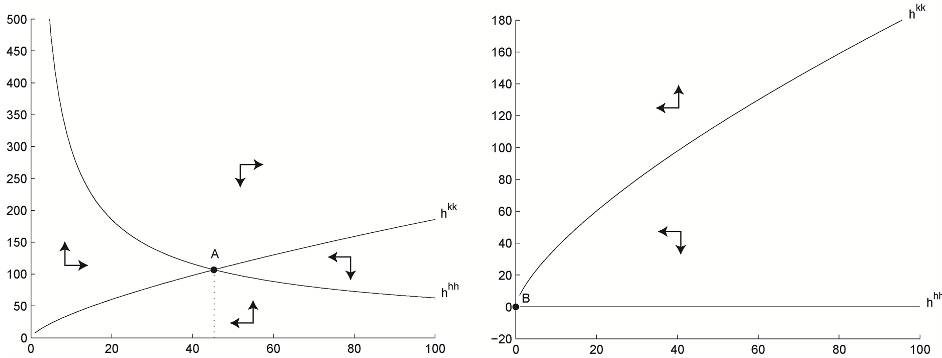
The dynamic systems at steady state explicit form are given by Equations (14) and (15) and the phase diagram of these are shown in Figure 1.
 (14)
(14)
 (15)
(15)
where, .
.
The arrows of motion under Assumptions 1 and 2 are attracting toward point A and attracting to point B in the area between the two curves and are respectively shown in Figure 1(a) and Figure 1(b)6.
 (a) (b)
Figure 1.
The phase diagram is constructed based on parameter values ,
, ,
, ,
, and
and . Human capital is on the y-axis and physical capital
is on x-axis. (a) Under Assumption 1
. Human capital is on the y-axis and physical capital
is on x-axis. (a) Under Assumption 1 . (b) Under Assumption
2
. (b) Under Assumption
2 .
.
Under Assumption 1, an interior solution for human and physical capital, point A in Figure 1(a), is given by Equations (16) and (17).
 (16)
(16)
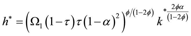 (17)
(17)
where,
 ,
,
 , and
, and
 in Equation (17) is given by Equation (16).
3.2. Stability
Based on parameter values outlined in Figure 1
it can be shown that point A in Figure 1(a) under
Assumption 1 is a saddle. Computing the Jacobian at
 produces the following real eigenvalues.
 (18)
(18)
where,
 represents the characteristic roots of the
polynomial
represents the characteristic roots of the
polynomial
 under Assumption 1. Furthermore, the elements of the Jacobian are derived from Equation
(13) whose map is defined as
under Assumption 1. Furthermore, the elements of the Jacobian are derived from Equation
(13) whose map is defined as . Given that the sum characteristic
polynomial evaluated at one is
. Given that the sum characteristic
polynomial evaluated at one is
 and evaluated at negative one
 ; it follows that the steady state
point
; it follows that the steady state
point
 is a saddle.
The steady state point under Assumption 2 is a sink. By assumption human capital
accumulation, Equation (8), has at minimum one unit of human capital for all insufficient
levels of both human capital,
 , and physical capital,
 . Such that steady state physical
and human capital poverty trap of Figure 1(b) has
. Such that steady state physical
and human capital poverty trap of Figure 1(b) has . Evaluating the steady state (point B in
Figure 1(b)) produces two positive and real characteristics
roots that lie within the unit circle
. Evaluating the steady state (point B in
Figure 1(b)) produces two positive and real characteristics
roots that lie within the unit circle .
.
3.3. Orbit and Bifurcations
Before exploring the size of the market failure the establishment of the behavior
in the neighborhood of the steady state
 under Assumption 1 needs to be established7.
In what follows the existence of a periodic orbit around the steady state point
and the steady state undergoing a bifurcation maintaining its orbit will be shown.
To simplify the analysis it is assumed that there are two types of households, poor
and rich households (as defined by ).
).
Let there be two types of households whose existence is based on Assumption 1 and
whose level of development is subject to the household type value of parameters.
To this it is said that there is a family of parameter values whose type is defined
in
 (i.e.
(i.e.
 poor household and
 rich household) such that
 is the value of a family of parameters by household type8. In an attempt to simplify
the dynamics and to maintain the model tractable the following assumption is made:
is the value of a family of parameters by household type8. In an attempt to simplify
the dynamics and to maintain the model tractable the following assumption is made:
Assumption 3 At equilibrium, (that is, at point A in Figure
1(a), given its parameter family value .)
.)
human capital
 is such that
 .
.
Assumption 3 states that around or at
 in some small neighborhood
 human capital is nonchanging. That is, additional knowledge is neither created nor
destroyed in the neighborhood
human capital is nonchanging. That is, additional knowledge is neither created nor
destroyed in the neighborhood . Such that the orbital map
 is one dimensional in physical capital.
Given Assumption 3 the nonlinear Equation can be rewritten as:
 (19)
(19)
where,
 is a
is a
 map and its solution
 is a saddle point solution at
 . Next consider an exposition of
the saddle-node bifurcation under a change in the parameter family
. Next consider an exposition of
the saddle-node bifurcation under a change in the parameter family
 that characterizes the two assumed level of developments. Let, the rich households
have a consumption discount preference in the first period of 0.6 and poor households
that characterizes the two assumed level of developments. Let, the rich households
have a consumption discount preference in the first period of 0.6 and poor households .9 Then a change in
 as defined by
 produces a saddle-node bifurcation. This is seen as a result of the hyperbolicity
around
produces a saddle-node bifurcation. This is seen as a result of the hyperbolicity
around . That is, Equation (19) is hyperbolic if none of its eigenvalues
are on the unit circle. From
. That is, Equation (19) is hyperbolic if none of its eigenvalues
are on the unit circle. From
 it is clear that none lie on the unit circle. This is also true after altering
 . Figure 1 provides diagram
of the above.
. Figure 1 provides diagram
of the above.
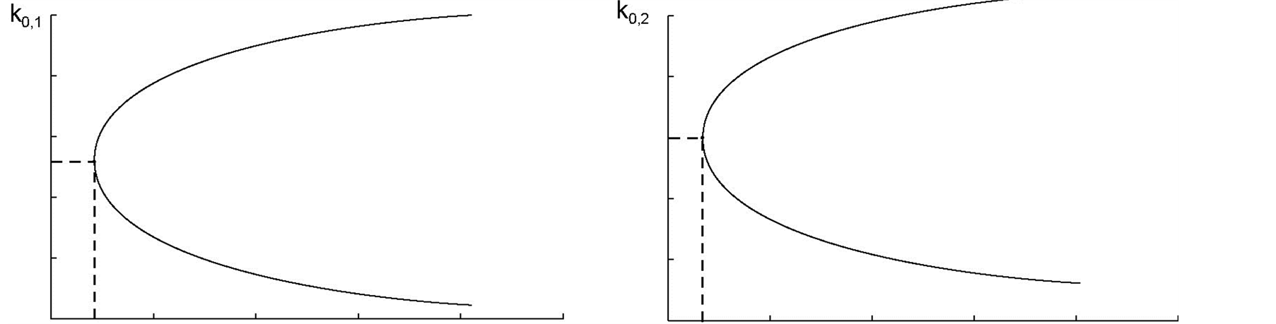
Figure 2(a) and Figure
2(b) show that under each household its solution to Equation (19),
 , has a family
 that is also its bifurcation value. That is, any changes to family
 experiences a bifurcation. Next the orbit around
 is evaluated.
Given the use of a discrete dynamic system it is clear that any orbit in some local
region
 in neighborhood
 is subject to chaotic behavior. However, based on the arrows of motion in Figure 1(a) while point A is not a sink it is nonetheless
stable near it. Whether the orbit is homoclinic and includes
is subject to chaotic behavior. However, based on the arrows of motion in Figure 1(a) while point A is not a sink it is nonetheless
stable near it. Whether the orbit is homoclinic and includes
 or a periodic orbit around
 is not of great concern here. For the purpose of this paper all that is needed is
the existence of at least one orbit
is not of great concern here. For the purpose of this paper all that is needed is
the existence of at least one orbit
 that shows properties of stability. However, the stability need not be on the orbit
but rather on the
that shows properties of stability. However, the stability need not be on the orbit
but rather on the
 region in
 . To this it is known
that at least one such region exists based on the arrows of motion. Let this
region in
. To this it is known
that at least one such region exists based on the arrows of motion. Let this
region in
 be defined as
 such that
 that is defined under Assumptions 1 and 3 is locally stable. Furthermore, the region
 in the local neighborhood
 is identical in size to the area around
 and
and
0.34 0.32
 (a) (b)
Figure 2. Bifurcation point
for poor and rich households is reached at
 respectively. (a) and (b) show the bifurcation diagram of Equation (19) where
 is in the y-axis and a range of
 around
 for poor and rich household’s in the
 -axis.
 . This states that in
 there is a periodic point
 around
 that is equal in distance
 (i.e.
(i.e.
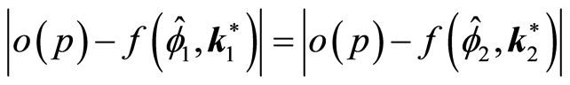 ). For simplicity let the positive and negative
periodic points be of equal distance from
). For simplicity let the positive and negative
periodic points be of equal distance from .
.
The statement of distance is quite reasonable since under bifurcations undertaken
by
 the eigenvalues, stability, and arrows of motion do not change as a result of the
location change in
the eigenvalues, stability, and arrows of motion do not change as a result of the
location change in . That is, the changes in
 are location changes and not changes in the mass of the steady state point. Let
the following proposition be a summary of the above:
are location changes and not changes in the mass of the steady state point. Let
the following proposition be a summary of the above:
Proposition 1 The positive and negative periodic point in the region around
 within the stable subspace
 is of equal distance in the dimension of
 ,
,
 .
.
4. Market Failure
The analysis of the size of the market failure is subject to the following definition:
Definition 1 (Market Failure) At the saddle point
 there exist a set of public-goods contracted quantity
 and price
 such that
 and constant at
 . The size of the market
failure is therefore defined as the change in
. The size of the market
failure is therefore defined as the change in
 (i.e.
(i.e. ) that results from
 at the periodic point
 in
in
 (i.e.
(i.e. ).
).
 as shown in Equation (4) can now be written as:
 (20)
(20)
The public-goods producer will generate output
 and pay labor and capital services based on Equations (2) and (3). In addition,
given Definition 1 and Equation (20) the value of
and pay labor and capital services based on Equations (2) and (3). In addition,
given Definition 1 and Equation (20) the value of
 at
at
 is known. That is, at period
 , where
 is a known value public-good prices are set and some normal level of
 is observed and agreed upon by all parties10.
Therefore,
 defined by Equation (20) and given Definition 1
states that the size of the market failure is the effect on
defined by Equation (20) and given Definition 1
states that the size of the market failure is the effect on
 given
given
 at periodic point
 in
in
 whose deviation is measured from
 .
.
This simply states that the size of the market failure is the difference between
what the government and the public-goods producer agreed were the costs of production
and what it ultimately cost to produce at the time of delivery. Under a perfect
markets scenario this difference would be internalized and no system of bureaucrats
be necessary (i.e. ).
).
4.1. The Poor and Rich
Poor and rich households have already been defined over the parameter value set . Consider then, the size of the market failure given these
two levels of development.
. Consider then, the size of the market failure given these
two levels of development.
Proposition 2 (a) The size of the market failure is larger in Poor households than rich ones.
(b) Poor households have higher variance in market failure than do rich ones.
Proof. The proof to Proposition 2 is easier found my numerical computation. For
instance, Proposition 2(a) is found by showing that . For simplicity, let the
periodic point in its outer range from center in
. For simplicity, let the
periodic point in its outer range from center in ,
,
 , be one unit away from
 . Such that, using the parameter
values employed in the previous section for poor and rich households generates
. Such that, using the parameter
values employed in the previous section for poor and rich households generates
 and
and
 respectively.
In addition, the spread between
 and
and
 also decreases as a household moves to a higher level of development (Proposition
2 (b)). That is, for an equal number of randomly allotted periodic points
also decreases as a household moves to a higher level of development (Proposition
2 (b)). That is, for an equal number of randomly allotted periodic points
 in
in
 within
 each household type generates sets of
 that produces the set of market failure size points
 that are decreasing in variance as a household moves from low to higher levels of
development. Given the parameterized model this implies
that are decreasing in variance as a household moves from low to higher levels of
development. Given the parameterized model this implies
 for poor and rich households respectively. Or a reduction in variance of about 0.01
as one moves from the poor to the rich economies steady state.
for poor and rich households respectively. Or a reduction in variance of about 0.01
as one moves from the poor to the rich economies steady state.

4.2. Theory versus Data
The theoretical model presented above provides a number of specific findings.
Implication 1 Poor households will have higher levels of corruption relative to more developed households.
Implication 2 Poor households will have higher variance in corruption levels than developed households.
Implication 3 Corruption abatement can only take place if the household moves to a higher steady state.
Implication 4 Corruption is a map and not a point.
Implication 5 Higher levels of human capital are present in more developed households and hence higher levels of human capital are associated with less corruption.
Figure 1 in [1] (page 435) shows growth rate in the y-axis and perception of corruption in the x-axis. Their figure is telling of Implications 1 and 2 in that it clearly shows a negative regression line in the level of perceived corruption to economic growth (See also [8] ). Moreover, it also shows a greater dispersion (variance) of growth levels at the higher units of perceived corruption.
In addition, in [4] figure 3 they show a u-shaped relationship between income and benefit of government intervention. The argument is that in poor countries there is a higher opportunity costs associated with diverting scarce resources to bureaucratic monitoring. This suggests that in poor countries one expects to see higher incidences of corruption.
Implication 3 is what this paper terms the [9] paradox. This implication provides a good interpretation as to why institutional reform (corruption abatement) in less developed nations has not led to lasting development. The present theory states that reform aimed at producing sustainable economic development must target individuals’ preferences and not institutions. This is quite a strong statement since it suggests that the chicken and egg question is no question at all rather that preferences are what define existent institutions and not the other way around. From a practical stance it is clear that both are important determinants of a successful development policy.
[4] introduces a system of bureaucrats and shows that there exists a socially optimal level of corruption. This work extends their findings by showing that there exists a map of corruption points that corresponds to a given level of development (as summarized by Implication 4).
Implication 5 is consistent with the findings in [1] [7] that show negative correlation between proxies of corruption and proxies of human capital. This implication is also consistent with the literature that link (negatively) corruption to growth ([1] [3] [8] ).
5. Conclusions
This paper has presented an alternative theoretical interpretation of market failures. It has been shown that the size of the market failure is produced naturally by the dynamics of an economy. The findings of the model showed that levels and dispersion of market failure and hence corruption at any given level of development can be found independent of a model that incorporates a system of bureaucrats.
Using a two-period OLG model the paper developed a full set of dynamical implications and showed that theoretically corruption is associated with a given level of development. Most importantly, it was not development per se that led to market failure rather it was the full set of priors that determined both the level of development and the size of the market failure. This has important implications to the development literature. As the present theory suggests, corruption abatement policies that ignore the dynamic forces of an economic system will not work.
The findings of the theoretical model are consistent with a large body of the corruption empirical and theoretical literature. This paper provided an alternative approach to view the cause of the observed corruption findings in the literature.
References
- Pellegrini, P.L. and Gerlagh, R. (2004) Corruption’s Effect on Growth and Its Transmission Channels. Kyklos, 57, 429-456. http://dx.doi.org/10.1111/j.0023-5962.2004.00261.x
- Jain, A.K. (2001) Corruption:
A Review. Journal of Economic Surveys, 15, 71-121.
http://dx.doi.org/10.1111/1467-6419.00133 -
Mauro. P. (1995) Corruption and Growth. The Quarterly Journal of Economics, 110,
681-712.
http://ideas.repec.org/a/tpr/qjecon/v110y1995i3p681-712.html - Acemoglu, D. and Verdier, T. (2000) The Choice between Market Failures and Corruption. American Economic Review, 90, 194-211. http://dx.doi.org/10.1257/aer.90.1.194
- Rose-Ackerman, S. (1975) The Economics of Corruption. Journal of Public Economics, 4, 187-203. http://ideas.repec.org/a/eee/pubeco/v4y1975i2p187-203.html
- Emerson, P.M. (2006) Corruption, Competition and Democracy. Journal of Development Economics, 81, 193-212. http://ideas.repec.org/a/eee/deveco/v81y2006i1p193-212.html
- Mocan, N. (2008) What Determines Corruption? International Evidence from Microdata. Economic Inquiry, 46, 493-510. http://dx.doi.org/10.1111/j.1465-7295.2007.00107.x
- Fisman, R. and Svensson,
J. (2007) Are Corruption and Taxation Really Harmful to Growth? Firm Level Evidence.
Journal of Development Economics, 83, 63-75.
http://dx.doi.org/10.1016/j.jdeveco.2005.09.009 - Easterly, W. (2000) The Elusive Quest for Growth. MIT Press, New York.
- Aidt, T.S. (2006) Economic Analysis of Corruption: A Survey. The Economic Journal, 113, F632-F652. http://dx.doi.org/10.1046/j.0013-0133.2003.00171.x
- North, D.C. (1990) Institutions, Institutional Change and Economic Performance. Cambridge University Press, New York. http://dx.doi.org/10.1017/CBO9780511808678
- De Soto, H. (2000) The Mystery of Capital. Basic Books, New York.
- Le, N.H. (1964) Economic Development through Bureaucratic Corruption. American Behavioral Scientist, 8, 8-14. http://dx.doi.org/10.1177/000276426400800303
- Levitt, S.D. and Dubner, S.J. (2005) Freakonomics: A Rogue Economist Explores the Hidden Side of Everything. Harper Collins, New York.
- Olken, B.A. (2006) Corruption and the Costs of Redistribution: Micro Evidence from Indonesia. Journal of Public Economics, 90, 853-870. http://ideas.repec.org/a/eee/pubeco/v90y2006i4-5p853-870.html
- Hodgson, G.M. and Jiang, S. (2008) The Economics of Corruption and the Corruption of Economics: An Institutionalist Perspective. Journal of Economic Issues, 41, 1043-1061.
- Easterly, W. (2008) Design and Reform of Institutions in ldcs and Transition Economies. American Economic Review: Papers & Proceedings, 98, 95-99. http://dx.doi.org/10.1257/aer.98.2.95
- Olken, B.A. (2007) Monitoring Corruption: Evidence from a Field Experiment in Indonesia. Journal of Political Economy, 115, 200-249. http://ideas.repec.org/a/ucp/jpolec/v115y2007p200-249.html
- Ghiglino, C. (2002) Introduction to a General Equilibrium Approach to Economic Growth. Journal of Economic Theory, 105, 1-17. http://ideas.repec.org/a/eee/jetheo/v105y2002i1p1-17.html
NOTES

1 evaluates the effects of corruption on firm growth in Uganda.

2 uses a proxy measure of corruption that has positive values of corruption for all 49 countries in his sample.
3Early work by argues that corruption is a an effective way of allowing markets to clear where otherwise transactions would fail to take place. Similarly, shows that there is a strong argument to be made for efficient levels of corruption.
4 uses a more direct way to capture corruption as the difference between government allotted rice to villages and household reported rice consumption.

5Work by further claims that top down institutional change policies are highly unlikely to succeed. The work by provides at least one case where top down monitoring reduces observed corruption. However, does not tie decreased corruption with long-term development.

6 above and
 below while
 below and
 above steady state.

7In what follows the special case of Assumption 2 and its dynamics are ignored. This case can be taught as a failed state (e.g., Somalia) and it is hard to justify theoretically that there exists a neighborhood of the poverty trap that will generate positive levels of growth even with small perturbations.

8This assumption states that rich households are expected to have slight differences in preferences. For instance, one can argue to poorer households relative to rich households are likely to have a higher first period consumption discount preference.
9See for a discussion on consumption time preferences and its effect to the level of development. Note that in the present model there is no population heterogeneity. That is, the heterogeneity exists across economies and the current analysis of rich and poor household are meant to capture rich and poor economies.

10Alternatively, one can think of government and the public-goods producer
agreeing on the price level for public goods given the information acquired by the
average physical capital level . This states that in the local neighborhood
 the entire set of periodic points
 that define the local stable neighborhood in
 produces a set of state values
 whose average is simply
 .
.