ABSTRACT

To date, most studies of firm concentration have considered local markets and as a consequence they have exploited market size as a key determinant of the number of firms. We consider instead the case of intermediate goods producers, specifically agro-food processors, whose markets may be regional, national, or even international. For such firms the extent of their markets is indeterminate. However, changes in the size of their markets are likely slowly evolving—thus suggesting that changes in firm counts can condition out demand effects. This study proposes a new estimator for the analysis of firm level turnover that employs changes in firm counts over a period of observation. The empirical model has several attractive features: it can be applied to secondary data on firm numbers, it can accommodate differenced integers, it can produce expected levels of entry and exit in a particular market, and it can be extended to a multivariate system. An application to modeling changes in numbers of dairy processors in four regions of western France suggests the merit of the econometric approach.

Keywords:Firm Entry, Firm Exit, Heine Distribution, Discrete Normal, Differenced Integers

1. Introduction

To date, most studies of firm concentration have considered local markets (e.g., [1] -[4] ) and as a consequence they have exploited market size as a key determinant of the number of firms. We consider instead the case of intermediate goods producers, specifically agro-food processors, whose markets may be regional, national, or even international. For such firms the extent of their markets is indeterminate. However, changes in the size of their markets are likely slowly evolving—thus suggesting that changes in firm counts can largely condition out demand effects. Another advantage of using changes in firm numbers rather than modeling entry and exit separately is that this sharply reduces data requirements. Observations on the number of new firms which enter and the number of incumbent firms which exit the market comprise data that are typically not available from secondary sources [5] . In fact there may be no clear consensus on what constitutes entry and exit even when microdata are available [6] . Lastly, the economic measures which affect entry and exit decisions are rarely observed for individual firms. For incumbent firms, cost and sales data may be considered proprietary, whereas the firm itself may not even be able to quantify measures such as goodwill or salvage value. Potential entrants (assuming that they could be identified) on the other hand would form expectations regarding profitability and entry costs. Collection of these expectations is certainly problematical.

Empirical analyses of the numbers of firms in narrow, geographically defined markets commonly have employed total firm counts (e.g., [1] [2] [7] ) and cross-sectional units of observation. This approach turns on the notion that by incorporating information on market context, such as population and per capita income, threshold levels of firm concentration can be estimated. By extension, opportunities for entry or exit can be quantified. However, cross-sectional units of observation can muddle the quantification of market context. Each market has its own unique features that may be unobserved or difficult to measure. To account for this individual heterogeneity, either differenced data or panel data are needed. Yet discrete statistical models of firm counts are not easily extended to handle differenced counts or a panel of counts.

Several important studies have embraced frameworks based on dynamic discrete games. Aguirregabiria and Mira (A & M) [4] developed an empirical model of players’ (firms’) belief about the behavior of their competitors and attempted to solve for a unique optimal decision representing each firm’s best response. Pakes, Ostrovsky, and Berry (POB) [8] similarly posit that firms form perceptions of the behavior of incumbents and potential entrants such that in equilibrium these perceptions become consistent with the distribution generated by the observed behavior. More recently, Abbring and Campbell [9] have extended the work of Bresnahan and Reiss [1] under the assumption that thresholds determine the entry and exit decisions of all firms.

Microeconometric analysis of firm turnover has used market size as a fundamental determinant of firm counts ([1] -[4] ). Our application to agro-food processors represents an important departure from such analyses. We recognize that processors may be important employers in rural areas but rather than producing for a localized market, processors may distribute nationally and internationally. Consequently, the markets these firms supply may be difficult to identify. Location is more likely determined by labor availability, proximity to raw inputs, transportation, and other infrastructure. Some locational advantages may be difficult to observe. However if such characteristics change slowly over time, then they can be conditioned out by a time series analysis.

As in A &M [4] and POB [8] , this study’s estimator for the analysis of firm level turnover in geographic markets does not draw inferences from a single cross-section of market structure observations. The empirical model has several attractive features: it can be applied to secondary data on firm numbers, it can accommodate differenced integers, it can produce expected levels of entry and exit in a particular market, and it can be extended to a multivariate system. The estimator can be thought of as mimicking a discrete dynamic game in which all participants are identical. These notions are discussed in the following section before we develop the statistical underpinnings for the estimator.

2. Determinants of Turnover

Our focus is on the firm level dynamics which lead to entry and exit within a spatially defined market. Jovanovic [10] first incorporated firm specific stochastic shocks in a model of market equilibrium through exit and entry. Subsequent studies have also introduced heterogeneity in firm level profits [11] , in firm size and growth rates [12] , in firm-specific sources of uncertainty [13] , and in product choice [14] . These lines of research allow for differences among firms but they do so at the cost of making empirical modeling effectively infeasible. Breshnahan and Reiss [1] treat firms homogeneously and instead introduce heterogeneity across markets. It is our claim that single cross-sectional analyses are tainted by the unobserved or mis-measured characteristics unique to each market and hence cannot distinguish between competitive and agglomerative forces [2] .

Common elements from these studies suggest that at the beginning of each decision period the incumbent firm has some probability of exiting the market. This probability is affected by productivity and/or regulatory shocks, expectations of future profits, and the current salvage value of the firm. Potential entrants form probabilities of entering the market depending on expectations of future profits and costs of entry.

Of course, when deciding on entry any given firm is unaware of how many other firms will enter the market. Similarly, incumbents are uncertain of the number of new firm entries that will occur over the decision/observation period. Firm-specific differences in profitability depend on idiosyncratic differences in managerial expertise, customer service, and goodwill. Since a firm’s managerial expertise cannot be easily assessed by its competitors, we assume firms endogenously sort themselves during the observation period so that the greater the range in unobservables such as expertise and goodwill, the greater the degree of turnover.

3. Econometric Model

3.1. Entry and Exit Probabilities

Consider the constellation of firms that are potential entrants in a market. We assign to each potential entrant a probability of entry—the firm with the highest probability we denote p₁, the second highest we denote p₂, etc. Of course we do not observe these probabilities directly, so we assume the log odds of entering the market is given by

The ith firm’s probability of entry then is

. (1)

This probability is increasing both in α and in the proportion ρ. We will see that the specific functional form for this probability (and the probability of exit) and bounds on the parameters α and ρ will allow us to translate probabilities of entry (and exit) into counts of firms entering (and exiting) a market.

To motivate the specification of α and ρ, we assume the log odds of an incumbent of exiting the market is given by

The jth firm’s probability of entry then is

(2)

Clearly, exit and entry probabilities are related since they share the two common parameters α and ρ. Note that the incumbent’s probability of exit is decreasing in α and increasing in ρ. The probability of entry or exit will be determined by the state of nature that the potential entrant or incumbent draws at the beginning of each decision period. The setup is similar to that developed by Abbring and Campbell [9] where firms observe market size and the number of firms operating in the previous period-these are the firms’ “inherited” values. Just as in Abbring and Campbell [9] , firms are named, i.e. they are indexed by i and j.

Since both α and ρ can be parameterized to depend on conditioning variables, the linkage between the probabilities is not as restrictive as might be thought. Further, the hyper-parameters permit an interpretation based on the linked specification of entry and exit probabilities. The proportion ρ can be considered as an index of turnover or churn because both probabilities are increasing in ρ. Therefore ρ might be parameterized to depend on variables related to technological or regulatory change, measures reflecting entry costs and salvage values, and the size of the market. On the other hand, higher values of α increase entry probabilities but decrease exit probabilities. Thus α might be parameterized to depend on measures related to profitability such as population growth, income growth, and firm density [3] . In this manner, the countervailing forces which are associated with positively and negatively correlated rates of entry and exit can be introduced.

3.2. Numbers of Firms Entering and Exiting

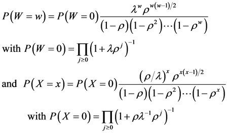
These probabilities, p_i and r_i, are related to counts of firms entering and exiting the market by assuming that each firm performs a Bernoulli trial by drawing from a uniform distribution with the probability of success given by the Bernoulli probability parameter, p_i or r_i, to determine whether it makes a move. The infinite sum of these independent Bernoulli random variables then is distributed as a Heine random variable [15] . These counts will be finite random realizations for a given α and ρ because as i→∞, p_i→0 and r_i→0. Denote the number of firms that enter a market over the observation period as w and the number of firms that exit the market as x. Then the probability mass functions for the random variables W and X are [15]

(3)

Setting λ = exp(α) and γ = ρ/exp(α), the means of the distributions are obtained as ([15] )

. (4)

The means are increasing in δ, γ, and ρ; however note that γ = ρ/λ so that depending on the sign of α, E[W] (E[X]) will be increasing (decreasing) in λ(γ) or decreasing (increasing) in λ(γ).

We illustrate the relationship between entry and exit probabilities and the corresponding Heine distributions in Table 1. The hypothetical values of α and ρ generate the probability series according to Equations (1) and (2).

For a potential entrant the probability of entering the market depends on the state of nature it draws (its p_i). Because there can be an infinite number of potential entrants, the expected number of entrants is the sum of these probabilities. This expectation is identically the expected value of the corresponding Heine random variable given in Equation (4). A similar setup holds for exit probabilities.

At this point if cross-sectional market data were available on the number of firms entering and exiting each market along with relevant conditioning variables, these distributions could be directly estimated via maximum likelihood methods. But as mentioned earlier, without a differenced or panel data model it is problematic to ac

count for market heterogeneity. Our solution is to entertain a differenced data model defined over two time periods (0,1) such that N₁ = N₀ + W − X and ΔN = W − X = Y. Total firms, N, by industry are available over time for many markets (e.g., NAICS data). Although we likely do not observe W and X, we do observe the random variable Y that is their difference. Fortunately the difference of two Heine random variables under the specification above is known to be distributed as discrete normal [16] . That is, by rewriting the probability mass functions (pmfs) in (3) as

, (5)

Kemp [16] proved that Y = W − X has the discrete normal distribution.

Kemp [16] characterized the discrete normal pmf of this difference of two counts as

. (6)

Note that the numerator of the pmf has as its argument the realization of the random variable (y) while the denominator is simply a normalizing factor that is summed over the support of the distribution, Y. Kemp [16] recognized that the discrete normal distribution i) is analogous to the normal distribution in that it is the only two-parameter discrete distribution on (–∞, ∞) for which the first two moments equations are the maximum-likelihood equations; ii) is log-concave ([17] , p.27); and iii) has either a single mode or a joint mode spanning two adjacent integers.

3.3. Reparameterizing the Discrete Normal Distribution

Unfortunately, Kemp’s [16] characterization does not permit closed form expressions of the mean and variance of Y. We can recast the parameters l and ρ to permit a representation of the pmf in terms of parameters associated with the mean and variance. Let λ = ρ^0.5–μ where –∞ < μ < ∞. Now λ is strictly positive and increasing in μ. As a result,

and next we posit

.

This parameterization explicitly links the notion of turnover or churn to a parameter associated with variation because the proportion ρ varies directly with σ². After some algebra, the discrete normal may be represented as

(7)

where the Y in the denominator represents the integer support of the distribution (–∞ < Y < ∞) and we note that E(Y) ≈ μ and V(Y) ≈ σ². The original parameters may be recovered from the underlying parameterizations: and Szablowski [18] has established the identical relationship using a reparameterization based on infinite series.

While there do not exist, in general, closed form expressions for the mean and variance, the location and dispersion parameters, μ and σ², are the approximate mean and variance respectively. We say approximate because problems arise when σ²→0. Basically, in these situations, the available points of support are not sufficient to reproduce a mass function with mean and variance equal to μ and σ² respectively (see also [18] ). For σ² > 1, note that μ and σ² can effectively be considered the mean and variance of the discrete normal distribution (with accuracy better than about 10⁻⁴ using the bounds provided by Szablowski).

This distribution can be fit to differenced integer data by employing maximum likelihood estimation. Since the discrete normal distribution is a member of the exponential family, consistent and asymptotically normal estimators of the parameters may be obtained under distributional misspecification [19] . For a given observation, we can use the linear link μ = xβ, where x is a 1 × k row vector of conditioning variables and β is a column vector of unknown coefficients, because μ can take on any value. It may also be advantageous to parameterize σ² because it is directly related to ρ and inversely related to λ. In this case an exponential link can be used to insure that σ² is positive. Once estimation is accomplished then estimates of the original parameters λ, ρ, and γ can be recovered using the relationships

, , and . By Equation (4) the expected level of entry and exit can be in ferred for each observation.

3.4. Multivariate Discrete Normal Distribution

Changes in the number of firms in one industry may be related to changes in the number of firms in another industry due to clustering effects, jointness in production or consumption, or economies associated with transportation. Alternatively, if firms in an industry are categorized by size, changes in the number of firms of one size may be related to corresponding changes of other sized firms.

The univariate discrete normal distribution can be generalized to the multivariate case of m industries using the following representation for a single market-based observation

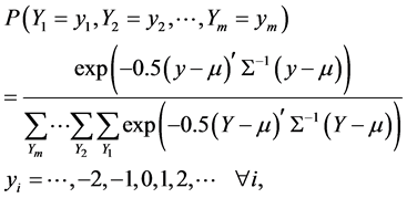(8)

where Σ is a positive definite symmetric matrix and quantities in bold denote m-element vectors. It can be shown that the multivariate discrete normal distribution is a member of the exponential family and has marginal discrete normal pmfs with corresponding parameters when the diagonal elements of S are sufficiently large. Maximum likelihood estimation over a sample on n markets is feasible when m is small or the region of support is compact.

4. Economic Rationale for the Application

As in A & M [4] , we assume that a market has N representative firms who compete in quantities and reach a static equilibrium in each period. The Cournot model that we adopt specifies a market demand of the form P = α – βQ and a market supply given by Q = Nq. Here q denotes the output of a representative firm in the market. The representative firm profit function may be written π = (P – c)q – k where c denotes marginal cost and k fixed costs. Profit maximizing output of the firm can be derived as and firm level profits under the Cournot solution are then

. (9)

Or more generally the variable profit function for a symmetric Cournot solution may be concisely written as

where θ is a function of marginal costs and the demand function and S represents market size [4] .

5. Empirical Application

5.1. Data and Model

We consider the number of milk and cheese processors in four regions of western France. This area, known as the Great West of France, possesses fertile lands, a temperate climate, and a diversified agricultural base. Studies of the pattern and distribution of the processors of agricultural commodities are still in a nascent stage ([20] [21] ). There is even less understanding of the dynamics of the creation and dissolution of agricultural processing firms. Using data from the National Institute of Statistics and Economic Studies (INSEE) we are able to trace individual milk and cheese processing firms over a twelve year period from 1996 through 2007. A firm is defined as an enterprise that employs at least 20 workers or has annual sales of over five million euros. Consequently our focus is on commercial enterprises that compete on the national, and possibly global, market. The data show relatively little variation in the number of firms with no discernable patterns that can be generalized across regions or industries.

Our response variables consist of the y_ijt which are the year-to-year changes in the number of firms (ΔN) in industry i (milk = 1; cheese = 2), region j (Lower Normandy = 1; Brittany = 2; Pays de la Loire = 3; and Poitou-Charentes = 4), in year t (t = 1997, ···, 2007). We estimate a two-industry bivariate system with 44 observations on each response variable. The specification of the hyperparameters μ and σ² is motivated by our previous discussion. Since μ is positively related to the number of new firms entering and negatively related to the number of incumbent firms exiting, we hypothesize that for each industry

. (10)

This specification reflects the assumption that firm entries are increasing—and conversely firm exits decreasing—in (the logarithm of) profits under the representative Cournot model. This follows the empirical modeling approach of A & M [4] . Notice that we do not include any measures of market size. This is in contrast to the studies by [1] [2] [4] where market size largely drives the empirical fit of their models. Because those studies analyze firms which operate in the retail and service sectors and serve local communities, market size is important. Our rationale recognizes that we are dealing with large firms producing intermediate goods; hence their effective markets are unknown.

Since σ² is positively associated with the firm turnover parameter, ρ, we hypothesize that for a given industry

(11)

Under the hypothesis that α₁ > 0, this formulation suggests that the amount of market turnover is positively related to the number of firms in the market. The policy variable is introduced to capture the reforms in the EU Common Agricultural Policy that were introduced in 2003. For the dairy sector in France, the consequence of these reforms was a gradual scrapping of the quota system that began in 2004. To capture this reform, the policy variable is defined to be zero prior to 2004 and its value is (year-2003)^1/2 in subsequent years to reflect the gradual abolition of the quota system. Since regulatory changes can introduce uncertainty, we hypothesize that α₂ > 0. Lastly, given that the diagonal elements of Σ are allowed to vary across observations, the off-diagonal element is specified as Σ_12t = κσ_1tσ_2t for each observation and κ has the interpretation of a correlation.

5.2. Empirical Results

The bivariate discrete normal model is estimated by maximum likelihood using MATLAB. Estimated parameters and their robust [22] standard errors are reported in Table 2.

^aFor parameters with double subscripts: 1 denotes Lower Normandy; 2 denotes Brittany; 3 denotes Pays de la Loire; 4 denotes Poitou-Charentes.

We are particularly interestedly in the sign and significance of the estimated β₁ parameters as they indicate whether our profitability measures derived from the Cournot model are relevant to these data. For both Industries we have established that our profitability measures are highly significant determinants of firm dynamics. With regard to the specification of our dispersion parameters—which are directly related to firm turnover—the results are somewhat mixed. While all α₁ and α₂ parameters are positive as hypothesized, they are not all highly statistically significant. We see that when the policy variable is highly significant, previous firm numbers are not, and conversely.

Joint estimation of the two industries does not yield a substantial increase in efficiency as indicated by insignificant correlation coefficient κ. Its positive value seems plausible by suggesting that within a region changes in one industry are positively related to changes in the other. The overall fit of the model can be assessed by predicting the y_ijt and calculating their correlation with the observed y_ijt response variables. These results are reported in Table 3.

It should be mentioned that one possible drawback to the empirical approach is that the normalizing factor, which comprises the denominator of the discrete normal pmf, allows a non-zero weight to be assigned to outcomes with exit levels that exceed the number of incumbents in the previous period. Logically the maximum number of exits in a time period is the number of incumbents in the previous period-since we do not allow for the possibility of firms entering and exiting in the same year. It is a simple matter to truncate the discrete normal distribution (see [23] ) to insure that implied exits cannot exceed the number of incumbents. To determine whether this is necessary, we estimate the univariate models for milk and cheese and compare these to their corresponding truncated models (where the truncation point is the negative of the number of incumbents in the previous period). For both univariate models the log likelihoods of the truncated versus the untruncated models were identical up to the third decimal place. Thus in this case there is no need to truncate the discrete normal distribution.

5.3. Recovering Implied Entry and Exit Levels

Because the discrete normal model is derived from two Heine distributions related to the unobserved levels of

^aAsymptotic p-value under alternative hypothesis that correlation is greater than zero.

new firm entries and incumbent firm exits, the estimated parameters from each discrete normal model can be used to recover these expected counts across firm types. For a given observation from an industry and region, the calculated levels of firm entry and exit are

and

.

We calculate the correlation between predicted entry and exit for each of the models and report these in Table 3.

6. Summary

Periodical counts of firms by rather detailed industry-type are easily obtained for markets as small as a county in the United States. Unfortunately such data are not informative as to the number of new firm entries or incumbent firm exits over the period of interest. However obtaining such detailed information is not a trivial matter and consequently systematic study of firm turnover is hampered by data requirements. And even if such data were available, analysis of it using modern models of firm dynamics [24] may not be feasible due to Syverson’s [3] claim that “data-gathering empirical economists know how famously possessive firms are about their cost data” (p. 1189).

The discrete normal model of changes in firm counts can be applied to widely available secondary data—yet its parameters may be related to underlying processes which can represent new firm entry and incumbent firm exit. These processes are reasonably flexible in that turnover is characterized by two different forces. One force acts to promote firm entry and, pari passu, discourage exit (and vice versa), while the other force is associated with both increased (or decreased) entry and exit.

A data set consisting of four regions in western France is analyzed in an effort to discern how the numbers of milk and cheese processors have changed between 1997 and 2007. Conditioning variables have signs consistent with a priori notions based on how the components with which they are associated account for the levels of entry/exit and their variability. While model fits as measured by correlations between predicted and observed variables are not particularly high, given the lack of variability and the minimal informational requirements imposed, our results are highly encouraging.

The discrete normal results are used to calculate the unobserved levels of entry and exit for each market and firm type. While the current application considers data that are discretely distributed, the modeling approach may be generalized to continuously distributed data sets. This follows because the statistical derivation suggests that when the dispersion parameter is large enough one may adopt a model specification based on ordinary least squares regression as for continuous data—and the mean and variance processes would be specified according to the rationale developed for the discrete normal form.

Acknowledgements

Data collection provided by Monique Harel. Research supported in part by USDA NRICGP #2002-01815, Institut National de la Recherche Agronomique (INRA)-LERECO, Region Pays de la Loire, and the Georgia Agricultural Experiment Station. 

References

- Bresnahan, T.F. and Reiss, P.C. (1991) Entry and Competition in Concentrated Markets. Journal of Political Economy, 99, 977-1009. http://dx.doi.org/10.1086/261786
- Shonkwiler, J.S. and Harris, T.R. (1996) Rural Retail Business Thresholds and Interdependencies. Journal of Regional Science, 36, 617-630. http://dx.doi.org/10.1111/j.1467-9787.1996.tb01121.x
- Syverson, C. (2004) Market Structure and Productivity: A Concrete Example. Journal of Political Economy, 112, 1181-1222. http://dx.doi.org/10.1086/424743
- Aguirregabiria, V. and Mira, P. (2007) Sequential Estimation of Dynamic Discrete Games. Econometrica, 75, 1-53. http://dx.doi.org/10.1111/j.1468-0262.2007.00731.x
- Sutaria, V. and Hicks, D.A. (2004) New Firm Formation: Dynamics and Determinants. Annals of Regional Science, 38, 241-262. http://dx.doi.org/10.1007/s00168-004-0194-9
- Disney, R. Haskel, J. and Heden, Y. (2003) Entry, Exit and Establishment Survival in UK Manufacturing. The Journal of Industrial Economics, 51, 91-112. http://dx.doi.org/10.1111/1467-6451.00193
- Pipkin, J.S. (1993) A Partitioning Model of Urban Retail Structure. Geographical Analysis, 25, 179-198. http://dx.doi.org/10.1111/j.1538-4632.1993.tb00290.x
- Pakes, A., Ovstrovsky, M. and Berry, S. (2007) Simple Estimators for the Parameters of Discrete Dynamic Games , with Entry/Exit Examples. RAND Journal of Economics, 38, 373-399. http://dx.doi.org/10.1111/j.1756-2171.2007.tb00073.x
- Abbring, J.H. and Campbell, J.R. (2010) Last-In First-Out Oligopoly Dynamics. Econometrica, 78, 1491-1528. http://dx.doi.org/10.3982/ECTA6863
- Jovanovic, B. (1982) Selection and the Evolution of Industry. Econometrica, 50, 649-670. http://dx.doi.org/10.2307/1912606
- Berry, S.T. (1992) Estimation of a Model of Entry in the Airline Industry. Econometrica, 60, 889-917. http://dx.doi.org/10.2307/2951571
- Hopenhayn, H.A. (1992) Entry, Exit, and Firm Dynamics in Long Run Equilibrium. Econometrica, 60, 1127-1150. http://dx.doi.org/10.2307/2951541
- Ericson, R. and Pakes, A. (1995) Markov-Perfect Industry Dynamics: A Framework for Empirical Work. Review of Economic Studies, 62, 53-82. http://dx.doi.org/10.2307/2297841
- Mazzeo, M.J. (2002) Product Choice and Oligopoly Market Structure. RAND Journal of Economics, 33, 221-242. http://dx.doi.org/10.2307/3087431
- Kemp, A. (1992) Heine-Euler Extensions of the Poisson Distribution. Communications in Statistics—Theory and Methods, 21, 571-588.
- Kemp, A. (1997) Characterizations of a Discrete Normal Distribution. Journal of Statistical Planning and Inference, 63, 223-229. http://dx.doi.org/10.2307/3087431
- Johnson, N.L., Kotz, S. and Balakrishnan, N. (1997) Discrete Multivariate Distributions. John Wiley, New York,
- Szablowski, P.J. (2001) Discrete Normal Distribution and Its Relationship with Jacobi Theta Functions. Statistics & Probability Letters, 52, 289-299. http://dx.doi.org/10.1016/S0167-7152(00)00223-6
- Gourieroux, C., Monfort, A. and Trognon, A. (1984) Pseudo Maximum Likelihood Methods: Theory. Econometrica, 52, 681-700. http://dx.doi.org/10.2307/1913471
- Cohen, J.P. and Morrison Paul, C.J. (2005) Agglomeration Economies and Industry Location Decisions: The Impacts of Spatial and Industrial Spillovers. Regional Science and Urban Economics, 35, 215-237. http://dx.doi.org/10.1016/j.regsciurbeco.2004.04.005
- Chevassus-Lozza, E. and Daniel, K. (2006) Market Openness and Geographical Concentration of Agricultural and Agro-Food Activities. Canadian Journal of Regional Science, 29, 21-42.
- White, H. (1982) Maximum Likelihood Estimation of Misspecified Models. Econometrica, 50, 1-25. http://dx.doi.org/10.2307/1912526
- Kemp, A. (2006) The Discrete Half-Normal Distribution. International Conference on Mathematical and Statistical Modeling in Honor of Enrique Castillo, Ciudad Real, Spain.
- Pakes, A. and Ericson, R. (1998) Empirical Implications of Alternative Models of Firm Dynamics. Journal of Economic Theory, 79, 1-45. http://dx.doi.org/10.1006/jeth.1997.2358