ABSTRACT

Most existing theoretical studies on home market effects depend crucially on the assumption of increasing returns to scale technology. This paper studies the consequences of the absence of increasing returns to scale on home market effects by employing a constant returns monopolistic competition model. This paper demonstrates that home market effects can emerge or disappear depending on the magnitude of the elasticity of substitution and transport costs even in the constant returns model with firm mobility. In particular, a reverse home market effect can result when the elasticity of substitution is low and transport costs are high.

1. Introduction

Paul R. Krugman argued ([1], p. 955): “In a world characterized both by increasing returns and by transportation costs, there will obviously be an incentive to concentrate production of a good near its largest market, even if there is some demand for the good elsewhere.” This is known as the “home market effect” (HME).

Most existing theoretical studies on the HME depend crucially on the assumption of increasing returns to scale (IRS) and monopolistic competition (as in Helpman and Krugman [2])¹. The presence of IRS serves one purpose. It guarantees that free entry of firms drives profits to zero, thereby determining the number of firms endogenously. Although the mathematical tractability of monopolistically competitive models is improved by the assumption of IRS, it appears to be at odds with reality because in the real world most firms earn positive pure profits. Hence, the use of a monopolistic competition model without IRS may be more realistic for economic analysis.

In contrast, the theoretical robustness of the HME under a constant returns to scale (CRS) technology and monopolistic competition setup is still a much neglected issue. The present paper studies the consequences that the absence of IRS has on the HME.

The crucial departure of the model developed in this paper from Helpman and Krugman [2] is to allow differentiated goods produced under CRS technology so that firms have positive pure profits. To study the theoretical robustness of the HME using such a model, the present paper assumes that the total number of firms in the world is fixed and considers the impact of a changing relative country size on the international distribution of firms (or each country’s share of firms) within the fixed number of firms.

This paper demonstrates that the HME can emerge or disappear depending on the magnitude of the elasticity of substitution between differentiated goods and transport costs even in the constant returns model. In particular, we show that the opposite effect of the HME can emerge when the elasticity of substitution is low and transport costs are high.

In the theoretical literature on HMEs, Davis [7], Head, Mayer and Ries [8], Yu [9], and Larch [10] extend the model of Helpman and Krugman [2] by making additional assumptions and also find that the opposite effect of the HME can emerge. However, all these studies rely on the assumption of IRS to examine the HME. This paper will show that the assumption of IRS in the differenttiated goods sector is not essential for discussion of the HME even in models with firm mobility.

The remainder of this paper is structured as follows. Section 2 outlines the features of the model. Section 3 describes the equilibrium and presents the impact of a changing relative market size on the equilibrium share of firms. The final section concludes the paper.

2. The Model

One crucial assumption in the literature on the HME is the presence of fixed costs in the monopolistic goods sector. The novelty of our approach is that we eliminate the fixed costs from the model used in the literature and study the robustness of the HME by using this setup.

We assume a two-country world economy, with a home and a foreign country. The models for the home and foreign countries are the same, and an asterisk is used to denote foreign variables. There are two types of goods, horizontally differentiated goods and a single homogeneous good. The differentiated goods are subject to a monopolistically competitive market structure, whereas the market for the homogeneous good is perfectly competitive. Both the differentiated goods and the homogeneous good are assumed to be produced using a constant-returns technology that requires labor as the only input. The market for labor is perfectly competitive and perfect labor mobility is assumed within each country. The homogeneous good is assumed to be traded freely, whereas trade in the differentiated goods incurs transport costs. Monopolistically competitive firms exist continuously in the world in the [0,1] range, where each firm produces a single differentiated product. Monopolistically competitive firms are mobile across countries, but their owners are not. Hence, all profit flows are distributed to the immobile owners according to the holding shares. In addition, firms in the interval are located in the home country, and the remaining firms are located in the foreign country, where n is endogenous. Therefore, measures the home (foreign) country’s share of firms. Meanwhile, as in Helpman and Krugman [2], homogeneous goods producers are immobile across countries. The size of the world population is normalized to unity. We assume that in the home country, households inhabit the interval and those in the foreign country inhabit the interval, where s measures the relative size of the home country. Each household owns one unit of labor.

Preferences are defined over a homogeneous good, named Y, and over differentiated goods, named C. In this paper, the preferences of household in the home country are represented by the following utility function²:

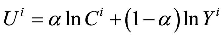(1)

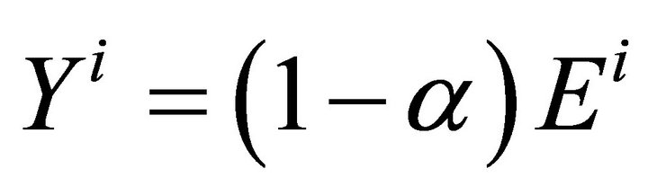
where a is the expenditure share on differentiated goods. Here, we take the price of the homogeneous good as the numéraire. Hence, the price is normalized to one. In addition, in Equation (1), the consumption index is defined as follows:

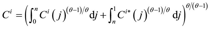, (2)

where measures the elasticity of substitution between any two differentiated goods and is the consumption of good j for household i. As in Helpman and Krugman [2], we assume iceberg transport costs in shipping the differentiated goods between countries. Specifically, units of a differentiated good have to be shipped from one country to the other for one unit to arrive at its destination. The consumption price indices are defined as:

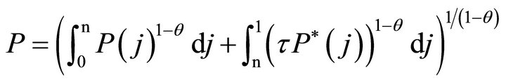, (3)

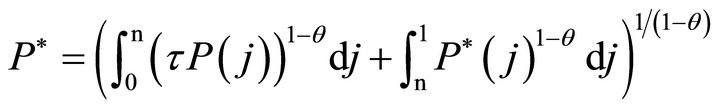, (4)

where is the price of differentiated goods produced in j. The value of expenditure for household i, , is defined as follows:

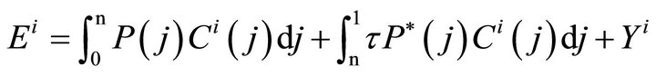. (5)

Then, the household budget constraint can be written as:

, (6)

where W denotes the nominal wage rate, g denotes the extent to which firms are owned domestically, and therefore,) is the nominal profit flow of firm j located at home (abroad).

Households in the home (foreign) country maximize (1) subject to a given level of expenditure (5) by allocating differentiated goods and optimally. This problem yields:

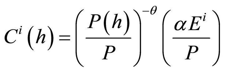, (7a)

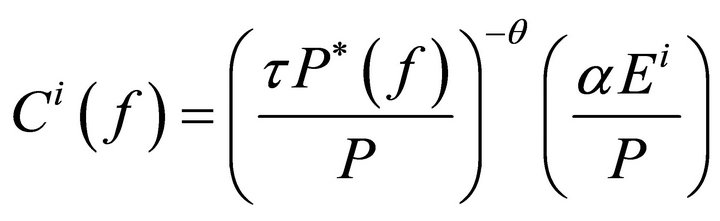, (7b)

. (7c)

Here, we define 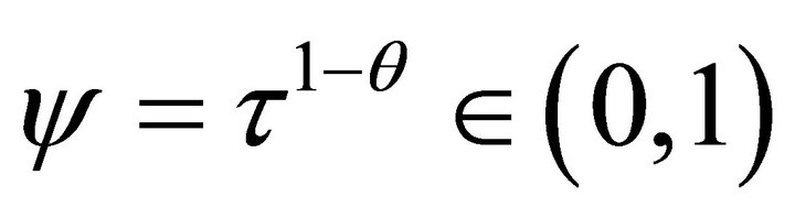as the degree of trade openness for convenience, where y equalizes to one under free trade and it also approaches zero when trade is extremely costly. The households are supposed to be symmetric, so we can delete the superscript i from. Aggregating the demands in (7a) and (7b) across all households worldwide yields the following market clearing condition for any differentiated product h, ³:

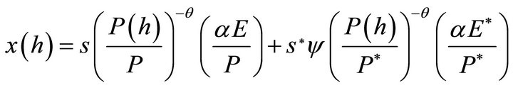. (8)

Similarly, for any product f of the foreign located firms, we obtain:

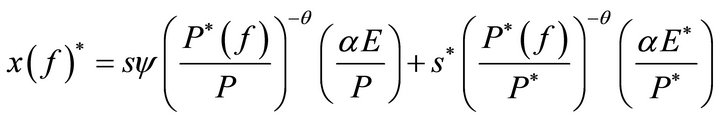. (9)

In the monopolistic goods sector, each firm has some monopoly power over pricing and one unit of labor is required to produce one unit of a variety. Because home-located firm h hires labor domestically, given W, P, E, and n, and subject to (8), home-located firm h faces the following profit-maximization problem:

.

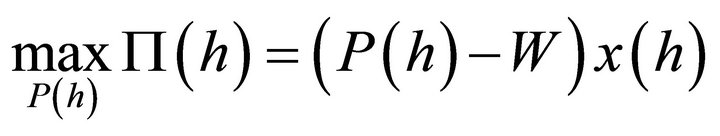By substituting from equation (8) into the firm’s nominal profit and then differentiating the resulting equation with respect to, we obtain the following price markup:

. (10)

Equation (10) tells us that a decrease in the value of q raises the markups of (11). This is because as the value of q decreases, the degree of monopoly increases.

Turning to the homogeneous good sector, one unit of labor is required to produce one unit of the homogeneous good. In addition, we assume that some production of the homogeneous good is active in both countries. Hence, the factor-price equalization across countries is ensured because of free trade of the homogeneous good. Therefore, from (10), we obtain:

(11)

Substituting (8) and (10) and those of foreign counterparts into the profit flows of the homeand foreign-located firms, and, respectively, we obtain:

, (12a)

. (12b)

The model assumes that firms do not face any relocation costs so that it does not take any time to relocate to another country. For a firm to be indifferent between home and foreign locations after location arbitrage, returns from the two locations must be equalized as follows:

. (13)

Here, substituting (11) into (3) and (4), respectively, we have

and.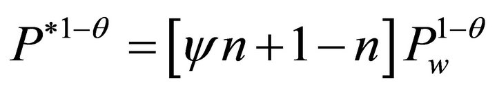

In addition, substituting these equations and (11) into (8) and (9), respectively, we obtain:

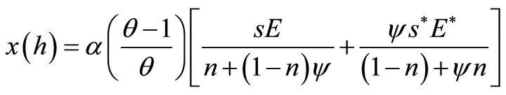, (14)

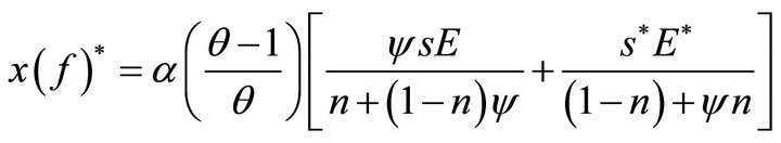. (15)

Furthermore, substituting (12a) and (12b) into (13), we obtain. If we substitute (14) and (15) into, we obtain:

(16)

Substituting (16) into (14) and considering, we obtain:

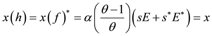. (17)

Substituting (12a) and (12b) into (13) and considering (17), we obtain:

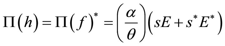. (18)

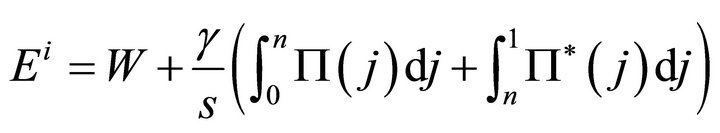
Substituting and (18) into (6) and because of, we have:

(19)

Similarly, for the foreign country, we obtain:

(20)

In the above equations, the first terms in the right hand side are wage incomes and the second terms are dividend incomes.

3. Market Equilibrium

From (19) and (20), we obtain sE and as:

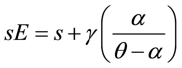, (21a)

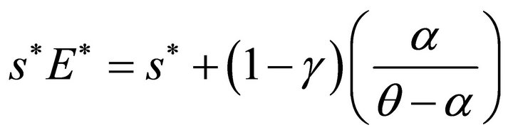. (21b)

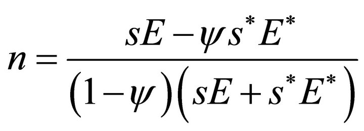
The above equations show that the total expenditures in two countries are increasing in the extent to which firms are domestically owned. Because an increase in g raises (decreases) the dividend incomes of the home (foreign) country. In addition, substituting (21a) and (21b) into (18), we obtain:

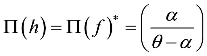(22)

From (22), the profit flows of firms decrease with the magnitude of the elasticity of substitution, regardless of its location. This is because a decrease in the value of q raises the markups of (11) so that the profits recorded in (22) increase. This offers the key to understanding why the reversed HME can emerge in the constant returns model. Furthermore, substituting (21a) and (21b) into (16) gives:

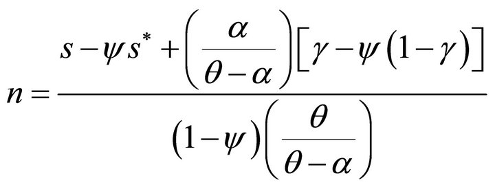⁴. (23)

From (23) and remembering, we find the parametric condition required for n to be between 0 and 1 (an interior equilibrium) as follows:

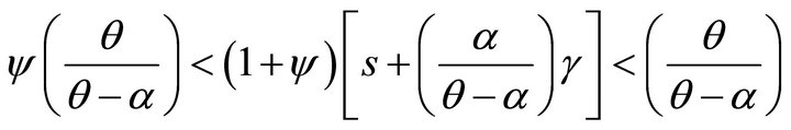. (24)

In what follows, we assume that (24) is valid, so that both countries produce the differentiated products. To explore the pervasiveness of HMEs in the constant returns model, following Head, Mayer and Ries [8], we focus on whether the share of distribution of firms increases or decreases disproportionately with the share of the country size, i.e., whether  exceeds or falls below one. If  exceeds one, the HME exists, i.e., the larger country has a disproportionally larger share of firms. Conversely, if  falls below one, the result is the opposite, i.e., the larger country has a disproportionally smaller share of firms. Substituting into (23), we obtain

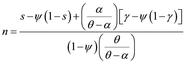. (25)

Taking the derivative of (25) with respect to s, we obtain:

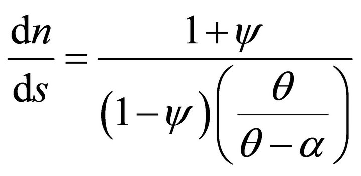. (26)

From (26), we obtain:

, when: inverse HME,                                                                         (27)

when: HME.                                                                                     (28)

From (27), when the elasticity of substitution is low (small q) and the transport costs are high (small y), the inverse HME appears: the larger the country size, the smaller the share of firms in that country5. This result also suggests that when the trade barriers and the degree of monopoly are high together, the inverse HME is likely to appear. Meanwhile, Equation (28) shows that the HME is observed as long as the elasticity of substitution is high enough (large q)6. This means that when the market structure is highly competitive, the HME is likely to emerge.

Intuitively, whether the constant returns model can exhibit the HME or the opposite effect of the HME depends on the relative strength of the centripetal and dispersion forces. The centripetal force is that firms are likely to locate in the larger country to reduce transport costs. Meanwhile, in our model, all profit flows are repatriated to the immobile owners of each country through dividends. Therefore, the dispersion force comes from the dispersed dividend incomes7. In addition, as shown in (22), the profit flows decrease with the magnitude of the elasticity of substitution. This implies that the dispersion force depends negatively on the magnitude of the elasticity of substitution. Hence, as q decreases, the dispersion force strengthens, and, consequently, this induces the opposite effect of the HME, as seen in (27). In contrast, when q is large enough so that positive pure profits are small, the dispersion force falls below the centripetal force, and, consequently, the HME emerges as seen in (28).

4. Concluding Remarks

So far, much recent theoretical work on the robustness of the HME is based on increasing returns to scale. This paper analyzed the question of whether or not the constant returns model exhibits the HME. The results indicate that when the elasticity of substitution of differentiated goods is high enough so that positive pure profits are small, the constant returns model can exhibit the HME. In addition, we also found that an effect opposite to the HME can result when the elasticity of substitution is low and transport costs are high.

5. Acknowledgements

The author would like to thank an anonymous referee for valuable comments. The author is also grateful to have received financial support from Tezukayama University.

REFERENCES

NOTES

¹For related works, see Weder [3], Crozet and Trionfetti [4], Behrens, Lamorgese, Ottaviano and Tabuchi [5], and Brülhart and Trionfetti [6].

²In what follows, we focus mainly on the description of the home country because the foreign country is described analogously.

³We have used the index h to denote the symmetric values within the home country, and we have used the index f for the foreign country.

⁴From (23), the symmetric equilibrium is always a solution when.

⁵Alternatively, Yu [9] defines the effect opposite to the HME as “the larger country ends up with a less-than-proportionate share of production of differentiated goods”.

⁶Incidentally, (26) shows that when, the proportionate equilibrium (i.e.,) is obtained.

⁷Note that in our model, there is a positive relationship between the repatriated dividend incomes and the local expenditures as seen in (6).