Journal of Mathematical Finance
Vol. 3 No. 1A (2013) , Article ID: 29347 , 10 pages DOI:10.4236/jmf.2013.31A019
Ex Post Efficient Set Mathematics
Sheffield University Management School, University of Sheffield, Sheffield, UK
Email: c.j.adcock@shef.ac.uk
Received January 9, 2013; revised February 12, 2013; accepted February 21, 2013
Keywords: Beta; CAPM; Efficient Frontier; Efficient Set Mathematics; Market Portfolio; Sharpe Ratio
ABSTRACT
This paper considers efficient set mathematics for the case where the covariance matrix of asset returns is assumed known but ex ante the vector of expected returns is replaced by an estimated or forecast value. It is shown that the ex post mean and variance differ from the standard results. Consequently the maximum Sharpe ratio portfolio also differs from the standard result. However, even with uncertainty about the vector of expected returns, subject to the assumptions made about the joint distribution of actual returns and estimated mean returns, ex post Sharpe ratio maximisers hold the ex post market portfolio. The properties of the zero beta portfolio are similar to the standard results leading to a capital market line. The ex post Capital Asset Pricing Model incorporates an intercept and the betas are not the same as those computed ex ante. The results are illustrated with an example.
1. Introduction
Portfolio selection introduced by Markowitz [1] has many supporters and many detractors. Broadly, the former are those who use his methods successfully and the latter are those who do not. Since its introduction, traditional portfolio selection has undergone much refinement and development. Nonetheless, many of these developments are very similar to or essentially identical to the original method. That is, a portfolio selector remains on a meanvariance efficient frontier. The original theory assumes a quadratic utility function or that the multivariate probability distribution of asset returns is characterized by expected returns and the covariance matrix. Stein’s Lemma, Stein [2], and its modern extensions (Liu, [3]; Landsman and Nešlehová, [4]) mean that these remarks are valid under a range of elliptically symmetric distributions and, subject to regularity conditions, for all utility functions. Thus, the efficient frontier should be a robust place to be.
In the previous paragraph, the phrase “a mean-variance efficient frontier” is used deliberately to remind that in practice all efficient frontiers are based on estimates of the underlying parameters, the vector of expected returns and the covariance matrix. Even when consistent estimators of the underlying parameters are used, all efficient frontiers are in reality estimated efficient frontiers. It is well known, by both practitioners and academic researchers, that the ex-post performance of an efficient portfolio often differs substantially from that anticipated at the time of construction. The celebrated papers by Best and Grauer [5] and Chopra and Ziemba [6] document that portfolios which are mean-variance efficient ex ante are sensitive to the inputs; that is to the estimators that are used. As Adcock [7] reports “even in the situation where the user is equipped with good estimates of the input parameters, the outputs are likely to produce results that are different from those expected. In circumstances where the estimates of the inputs are poor, it is inevitable that ex-post performance will be inferior”. The recent paper by Kan and Zhou [8] confirms this. These and other difficulties are documented widely, notably in Michaud [9,10].
The use of estimated values for the model parameters means that it is desirable, even necessary, to use statistical methods to study the behaviour of portfolios which ex ante are mean variance efficient. There is an early work due to Bawa, Brown and Klein [11]. In many papers, the starting point for the use of statistical methods in conjunction with mean-variance portfolio selection is often the work by Jobson and Korkie [12]. This work, in common with other later papers, is concerned with the maximum Sharpe ratio portfolio. If asset returns are IID normal and the usual sample estimators are used, Jobson and Korkie [12] show how to derive expressions for the expected values and variances of the components of the efficient frontier reported in Merton [13]. This version of the efficient frontier allows short positions; that is only the budget constraint is imposed on the expected utility maximization. The resulting formulae in Merton’s paper define the shape of the frontier and ex-ante portfolio expected return and variance. They are often referred to collectively as efficient set mathematics. Gibbons, Ross and Shanken [14] present a test of the mean-variance efficiency of a portfolio. This test, which employs a fundamental property of the efficient frontier, is based on a variant of the market model. Under the IID normal assumptions, it results in Hotelling’s T2, which apart from a scaling constant has an F distribution. There are similar tests in Huberman and Kandel [15] and Britten-Jones [16]. More recently, Kan and Smith [17] derive expressions for the joint distribution of the components of the efficient frontier given the standard assumptions. To achieve this, they reparameterise the frontier and consider components which are functions of those in Merton’s original representation. The results that they derive depend on the Chi-squared and non-central F distributions. Knight and Satchell [18] derive further extensions, specifically for institutional investors. There are several other related works, notably by Bodnar and Schmid [19-21], Hillier and Satchell [22] and Okhrin and Schmid [23].
Under the assumption that the vector of expected returns and the covariance matrix are known, the ex post or actual return on a portfolio is an affine transformation of the vector of asset returns. If returns follow a multivariate normal distribution or any member of the elliptically symmetric class, the distribution of portfolio returns is a member of the same class. The aim of this paper is to present results for the case where the covariance matrix is known, but the vector of expected returns is an estimate or forecast and is therefore a random vector. To avoid duplication, henceforth such a vector is referred to as a forecast. When the joint distribution of returns and the forecast used for portfolio selection is multivariate normal, it is shown that the distribution of ex-post portfolio returns is an extended quadratic form in normal variables. It is shown that this changes the shape of the efficient frontier and leads to different insights into the maximum Sharpe ratio or market portfolio. The results in this paper substantially extend those reported in Adcock [7,24,25].
The paper is set out as follows. Section 2 contains a summary of traditional efficient set mathematics and the assumptions used. Section 3 present the main results of the paper, namely that ex post returns are distributed as an extended quadratic form. Given that the number of possible specifications for the structure of the covariance matrix of asset returns and forecasts is large, Section 4 presents two examples. In Section 5, there are results which examine the effect of the estimated expected returns or forecasts on the Sharpe ratio, the market portfolio and the Capital Asset Pricing Model. Section 6 contains concluding remarks and a brief discussion of potential developments.
2. Traditional Efficient Set Mathematics
Let  be an n-vector of asset returns, which has the multivariate normal distribution
 . The notation
  denotes portfolio return and
  the risk free. The notations
 ,
,  and
and  denote respectively an n-vector of ones, an n-vector of zeros and an
  matrix of zeros. Subscripts are generally omitted. It is assumed that the covariance matrix
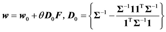
  is non-singular. Maximising expected utility subject only to the budget constraint in the usual way and recalling Stein’s Lemma, the first order conditions for portfolio selection lead to the well known expression for the portfolio weights
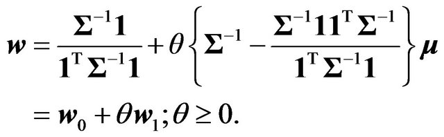
The vector  is the minimum variance portfolio and satisfies the budget constraint
 . The vector
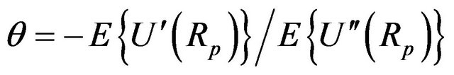
  is a self-financing portfolio. In general, risk appetite
  is defined as
The expected return and variance of portfolio return, which has a normal distribution given the assumptions, are

respectively, where the standard constants are defined as
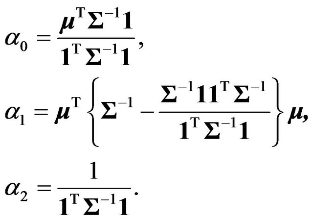
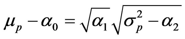
Note that these definitions of the standard constants differ from those in Merton [13]. They are the same as those used in Kan and Smith [17] and are more suitable for the purposes of this paper. The equation of the efficient frontier is
The market or maximum Sharpe ratio portfolio arises when
 as long as
 . If
. If  the market portfolio does not exist in any meaningful sense.
3. Distribution of Portfolio Returns
This section presents the main results of the paper, in which it is shown that when  is replaced by a forecast, denoted by
 , portfolio return is distributed as an extended quadratic form in normal variables. It is assumed the 2n-vector
 has a non-singular multivariate normal distribution
  with
with
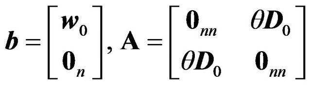
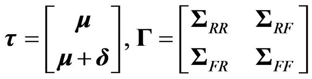 respectively. Non-zero entries in the vector
  mean that the forecast is biased. It is assumed that the covariance matrix is known. The vector of portfolio weights based upon the forecast
  is
is
Portfolio return is then
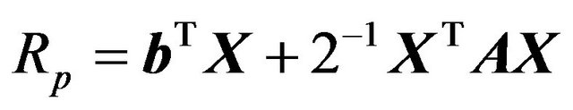 with
with
 .
.
Portfolio return is distributed as an extended quadratic form in normal variables. The properties of these are described in detail in Mathai and Prevost [26]. Relevant results for financial applications are in Appendix B of Adcock et al [27]. Specifically, Corollary 2 of their Theorem 2 leads to the following.
Proposition 1
Apart from an additive constant, portfolio return  is distributed as the weighted sum of independent noncentral Chi-squared variables, each with one degree of freedom, and an independently distributed normal variable. That is
where the  are the
  non-zero eigenvalues of the matrix
 ,
,  and
and  are scalar functions of elements of the vector
  and the eigenvectors of
  and
and  is a standard normal variable.
As further technical details of this result are not required for the material that follows below, they are omitted. Briefly, it may be noted that the probability density function of  is intractable, although the central limit theorem means that, ceteris paribus, the distribution of
  will tend to normality as the number of assets increases. This provides support to a finding of Tu and Zhou [28] who suggests that the normality assumption works for the evaluation of portfolio performance. The characteristic function of the extended quadratic form, however, may be inverted numerically using a procedure due to Imhof [29]. Mathai and Prevost [26] note that this procedure may be considered to be exact. The characterristic function is tractable and leads to the following results for the mean and variance of portfolio returns. An outline proof of the following proposition is in Appendix A. It was first reported without proof in Adcock [25].
Proposition 2
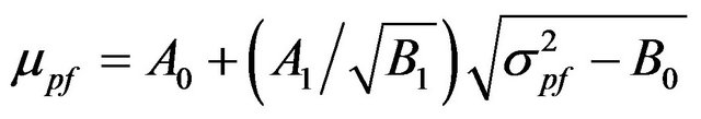
The expected value and variance of portfolio return, denoted with the additional subscript f, are respectively
where  and
and  are
are

and
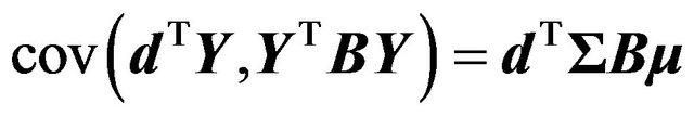
The covariance between the returns of an arbitrary portfolio with given weights  and an efficient portfolio with risk appetite
  is
is

Substitution gives the following:
Corollary 2.1
The equation of the efficient frontier is
 where
where
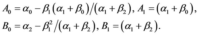
From Proposition 2 and Corollary 2.1, it is clear that the ex-post expected return and variance of an efficient portfolio constructed using estimates or forecasts of expected returns are different from those based on standard efficient set mathematics. The effect on the maximum Sharpe ratio portfolio is described in Section 5. The detailed effects on mean and variance, and hence the shape of the efficient frontier, depend on the constants . These in turn depend on
 , the bias in the estimates, and the structure of the covariance matrix
 . To illustrate the effects, two examples are presented in Section 4.
4. Two Examples
The matrices  and
and  may be written as
 where
where  and
and  are full rank
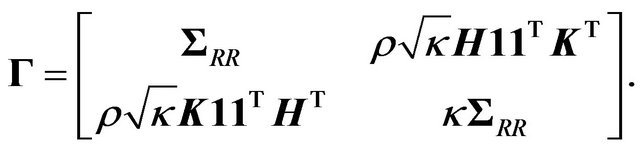
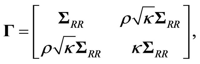
  matrices. The covariance matrix of returns and forecasts is
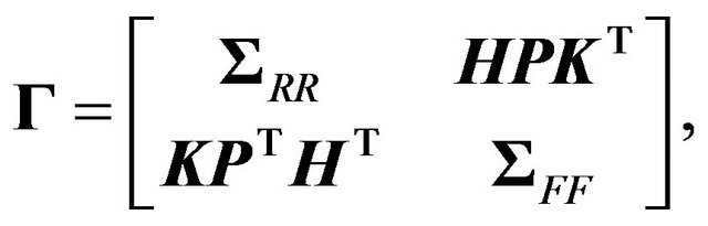
where  is the
  matrix of cross-correlations between returns and forecasts. It is convenient to define the following scalars

In the two examples below, it is assumed that the covariance matrix of the estimates or forecasts is proportional to , the covariance matrix of asset returns. This is loosely equivalent to assuming that the vector of forecasts is based on simple times series methods. It is also assumed that forecasts are unbiased,
 .
.
4.1. Rank One Cross-Correlation Matrix with Equal Correlations and Unbiased Estimates
In this case  which leads to
The constants  are
are
These are affected by the covariance matrix of asset returns through their dependence on . Note that 1) by the Cauchy Schwarz inequality
 , expected return is increased (decreased) if
  is positive (negative) and 2) that the requirement that
  be positive semidefinite imposes a restriction on
 .
.
4.2. Diagonal Cross-Correlation Matrix with Equal Correlations and Unbiased Estimates
This example was first reported in conference proceedings in Adcock [24]. In this case , where
  is the
  unit matrix, in which case
leading to

A special case of this is the use of the sample mean returns based on a time series of length . In this case
  and
and . There is no effect on mean return, but there is an increase in variance. In particular, the variance is an increasing function of the number of assets.
To illustrate these results a data set consisting of weekly returns from 13 FTSE indices is used. The forecast of the mean returns and the covariance matrix used are shown in Tables A1 and A2 of Appendix C. The illustration considers five values of correlation r = −0.05,−0.01,0,0.01,0.05. The parameter set for  corresponds to sample sizes of
 . The value
  may be interpreted as meaning that the covariance matrix associated with the forecasts is predictive, which corresponds with a sensible practice. The
  and
and  are computed using the formulae above. These are shown in Table 1. Panel 1) of Table 1 shows the standard constants. Panel 2) shows the computed values of
  corresponding to values of
  from −0.05 to 0.05. Note that the values of
  are two orders of magnitude greater than those for
 . In panel 3) the column entitled mult0 shows the multiplier to be applied to the Standard Sharpe ratio. Note that for
  the maximum Sharpe ratio occurs at a lower level of risk than the standard case, but that for
  the maximum Sharpe ratio portfolio is the minimum variance portfolio (MVP). A graph of the efficient frontier for 3 values of
 , namely −0.01, 0.01 and 0.05 and for
  is shown in Figure 1. The figure also includes a graph of the conventional efficient frontier. As the figure shows, when
  is less than zero the efficient frontier is downwards sloping: more risk leads to lower expected return.
Table 1. Parameters of the efficient frontier.
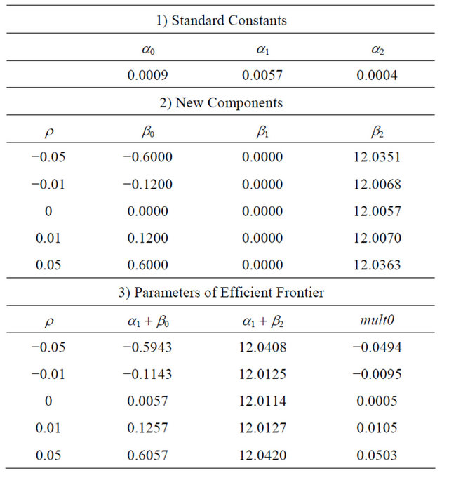
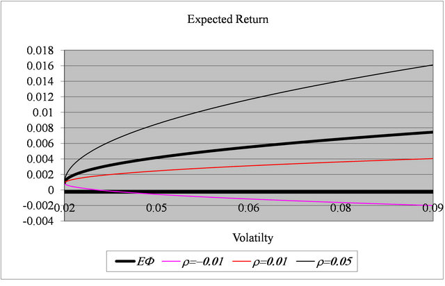
Figure 1. The efficient frontier based on forecasts.
For  the frontier is upwards sloping, but the gradient is always less than that for the ex ante efficient frontier. When
 , the gradient is higher. That is, this value of correlation provides a sufficient signal to outperform the ex ante frontier. To avoid cluttering the figure other values of
  are omitted. However, as
  increases so does the gradient of the frontier. Conversely as
  decreases from zero, the negative trade-off between risk and expected return becomes progressively worse.
The case  may be interpreted as the use of sample returns as a forecast is also omitted. In this case, the corresponding efficient frontier is effectively flat. Figure 2, which is in Section 5, shows the Sharpe ratios plotted against risk appetite
  for the same values of
  and for the ex ante case.
5. The Sharpe Ratio and the Market Portfolio
In standard efficient set mathematics, the Sharpe ratio is
 .
.
For  the maximum Sharpe ratio or market portfolio is given by
 . Sections 5.1 and 5.2 consider the Sharpe ratio and the market portfolio for the case when unbiased forecasts of
  are used, that is
 . Section 5.3 considers the distribution of returns on the conventional maximum Sharpe ratio portfolio for the case where the estimate
  is used in place of
 .
.
5.1. Properties of the Sharpe Ratio
Table 2 shows the differences between the standard Sharpe ratio and its properties compared with those when the effects of forecasts are taken into account. Specifically, in the rows labeled 1) the table shows the value of  that maximises the Sharpe ratio, in 2) the value of the Sharpe ratio at the maximum and in 3) the limiting value as
 . The corresponding results for the case of biased forecasts are substantially more complicated and
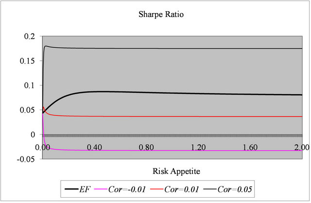
Figure 2. Sharpe ratios based on forecasts.
Table 2. Comparison of the sharpe ratio.
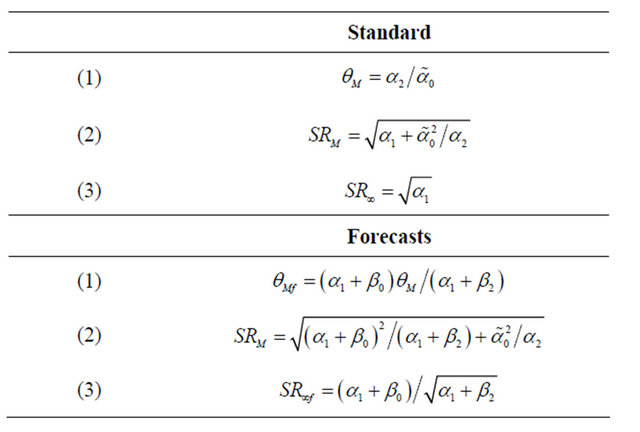
so are omitted, but are available on request. In the standard case, a necessary and sufficient condition for the maximum Sharpe ratio to exist in a meaningful sense is that . For the ex post Sharpe ratio the corresponding condition is
Figure 2 shows examples of the Sharpe ratio for r = −0.01, 0.01 and 0.05 and for . The standard Sharpe ratio is also shown. When r = −0.01 the maximum Sharpe ratio occurs at the MVP and the ratio declines monotonically as risk increases. For r = 0.01 the maximum is close to the MVP and the Sharpe ratio is always inferior to the ex ante case. When r = 0.05, however, the Sharpe ratio is superior to the standard case, but the maximum is attained at lower risk.
5.2. The Market Portfolio and the CAPM
The question of the market portfolio under forecast uncertainty naturally arises. Standard manipulations lead to the following.
Proposition 3
Given the assumptions above, the maximum ex post Sharpe ratio portfolio is the ex post market portfolio.
Thus, although the ex post market portfolio differs from that found ex ante, there is a corresponding capital market line, whose intercept is the risk free rate. The argument that investors will hold a combination of lending/borrowing and the market portfolio still holds. This is subject to the assumption that the joint distribution of returns and forecasts is the same for all market participants. This result leads in turn to the question of the CAPM. Under the assumptions of the paper, is the expected excess return on an asset or portfolio given by the product of beta and the expected excess return on the market portfolio? The treatment below follows that in Chapter 3 of Huang and Litzenberger [30] and requires the following result.
Proposition 4
The covariance of two efficient portfolios p and q is
 .
.
This leads to portfolio q being a zero-beta portfolio with respect to portfolio p if its risk appetite is
 .
.
Note that for the case where forecasts are biased  and portfolio p may be any portfolio including the minimum variance portfolio. For the case considered in detail in this section,
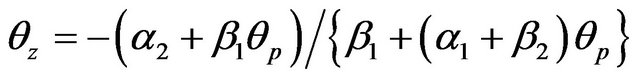
  and portfolio p can be any portfolio except the minimum variance portfolio. For this case, the expected return on the zero beta portfolio is
Standard manipulations, similar to those in Chapter 3 of Huang and Litzenberger, lead to the following
Proposition 5
The intercept of the straight line that is the tangent to the efficient frontier at portfolio p is equal to .
.
Proposition 6
If portfolio p is the market portfolio, the expected return on the zero beta portfolio equals the risk free rate .
.
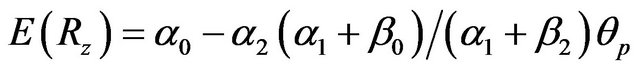
In the standard case where  is given, consideration of the covariance between the returns of portfolio p and an arbitrary portfolio leads to the CAPM if portfolio p is in fact the market portfolio. For the case considered in this paper, Proposition 2 leads to a modified version of the CAPM
Proposition 7
Let q be any portfolio with weights , M be the ex post market portfolio and let
  and
and  be their respective expected excess returns. When
 , it follows that
 where
where  is the beta of portfolio q with respect to M
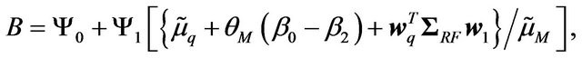
where
 .
.
Note that this reduces to the standard case when  is given, but that for this case the intercept is not zero in general.
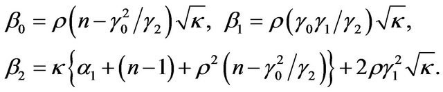
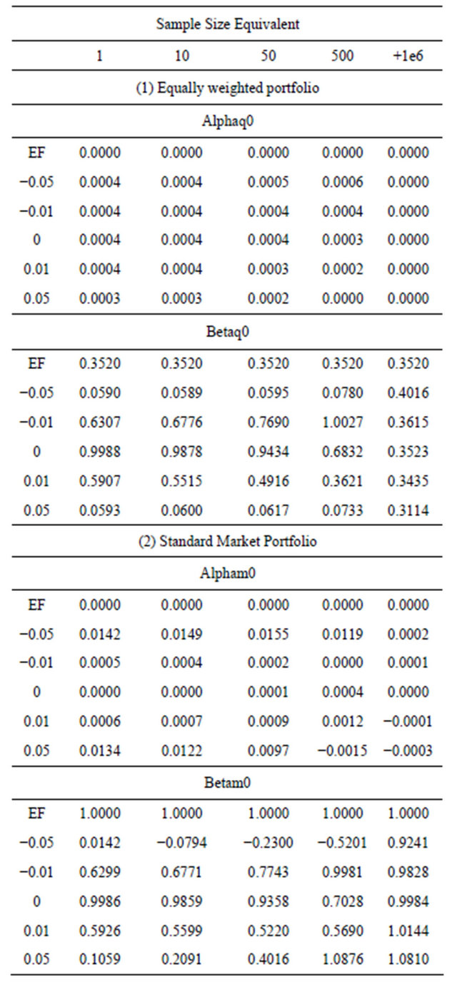
Continuing the example, Table 3 contains values of alpha and beta for two portfolios for the values of  and
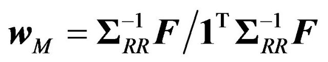
and  used above. The first portfolio is an equally weighted portfolio of returns on the 13 FTSE indices. The second is the conventional market portfolio for which the weights are proportional to
 . Panel 1) of Table 3 shows the alphas and betas for the equally weighted portfolio. These are computed for the standard efficient frontier (table rows called EF). They are also computed for the specified values of
  and
and . As the table shows, the values of alpha are non-zero. They are numerically small, but of comparable magnitude to the return forecasts shown in appendix Table A1. The values of beta decrease as
  increases. Both alpha and beta approach their standard values as
  decreases to zero, equivalently the implicit sample size increases. Similar behaviour is observed in Panel 2), although it is notable that the alphas are substantial when
 . It is also notable that beta is a non-linear function of both
  and
and , with the phenomenon being more apparent for the conventional market portfolio.
5.3. Property of the Maximum Sharpe Ratio Portfolio
When  is used as the forecast of expected return, the maximum Sharpe ratio portfolio has weights given by
 .
.
The return on the market portfolio is
 .
.
The following interesting result is proved in Appendix B.
Proposition 8
Given the assumptions above, the expected value of the market portfolio based on forecast of the expected return is undefined.
Strictly speaking, the result is of theoretical interest. Nonetheless, it suggests that returns on the maximum Sharpe ratio portfolio based on estimates may in practice be volatile.
6. Discussion and Concluding Remarks
This paper considers efficient set mathematics for the case where the covariance matrix of asset returns is as-
Table 3. Behaviour of alpha and beta.
sumed to be known but ex ante the vector of expected returns is replaced by an estimated or forecast value. It is shown that the ex post mean and variance differ from the standard results. Consequently the maximum Sharpe ratio portfolio also differs from the standard result. This portfolio remains the market portfolio. Thus, even with uncertainty about the vector of expected returns, subject to the assumptions made about the joint distribution of actual returns and estimated mean returns, ex post Sharpe ratio maximizers hold the ex post market portfolio.
The properties of the zero beta portfolio are also similar to the standard results. A notable exception, however, is that the capital asset pricing model incorporates an intercept and the ex post betas are not the same as those computed ex ante.
The numerical example provides a demonstration of well-known empirical features: positive correlations between returns and estimates improve ex post portfolio performance; negative correlations damage it; volatility ex post may be expected to be higher than that predicted ex ante.
The assumption of multivariate normality with known covariance matrix is a limitation of the results, except perhaps for those of low frequency. The results presented here imply that a tractable model for the multivariate probability distribution of returns and estimates is required. Scale mixtures of the multivariate normal distribution are an obvious candidate. The use of multivariate distributions which incorporate skewness is an open research question.
REFERENCES
- H. Markowitz, “Portfolio Selection,” Journal of Finance, Vol. 7, No. 1, 1952, pp. 77-91.
- C. M. Stein, “Estimation of the Mean of a Multivariate Normal Distribution,” Annals of Statistics, Vol. 9, No. 6, 1981, pp. 1135-1151. doi:10.1214/aos/1176345632
- J. S. Liu, “Siegel’s Formula via Stein’s Identities,” Statistics and Probability Letters, Vol. 21, No. 3, 1994, pp. 247-251. doi:10.1016/0167-7152(94)90121-X
- Z. Landsman and J. Nešlehová, “Stein’s Lemma for Elliptical Random Vectors,” Journal of Multivariate Analysis, Vol. 99, No. 5, 2008, pp. 912-927. doi:10.1016/j.jmva.2007.05.006
- M. J. Best and R. R. Grauer, “On the Sensitivity of MeanVariance-Efficient Portfolios to Changes in Asset Means: Some Analytical and Computational Results,” Review of Financial Studies, Vol. 4, No. 2, 1991, pp. 315-342. doi:10.1093/rfs/4.2.315
- V. Chopra and W. T. Ziemba, “The Effect of Errors in Means, Variances and Covariances on Optimal Portfolio Choice,” Journal of Portfolio Management, Vol. 19, No. 2, 1993, pp. 6-11. doi:10.3905/jpm.1993.409440
- C. J. Adcock, “Predicting Portfolio Returns Using The Distributions of Efficient Set Portfolios,” In S. E. Satchell and A Scowcroft, Eds., Advances in Portfolio Construction and Implementation, Butterworth Heinemann, Oxford, 2003, pp. 342-355.
- R. Kan and G. Zhou, “Optimal Portfolio Choice with Parameter Uncertainty,” Journal of Financial and Quantitative Analysis, Vol. 42, No. 3, 2007, pp. 621-656. doi:10.1017/S0022109000004129
- R. O. Michaud, “The Markowitz Optimization Enigma: Is Optimized Optimal?” Financial Analysts Journal, 1989, pp. 31-42.
- R. O. Michaud, “Efficient Asset Management,” Harvard Business School Press, Boston, 1998.
- V. Bawa, S. J. Brown and R. Klein, “Estimation Risk and Optimal Portfolio Choice,” Studies in Bayesian Econometrics, North Holland, Amsterdam, Vol. 3, 1979.
- J. D. Jobson and B. Korkie, “Estimation for Markowitz Efficient Portfolios,” Journal of the American Statistical Association, Vol. 75, No. 371, 1980, pp. 544-554. doi:10.1080/01621459.1980.10477507
- R. Merton, “An Analytical Derivation of the Efficient Portfolio Frontier,” Journal of Financial and Quantitative Analysis, Vol. 7, No. 4, 1972, pp. 1851-1872. doi:10.2307/2329621
- M. R. Gibbons, S. A. Ross and J. Shanken, “A Test of the Efficiency of a Given Portfolio,” Econometrica, Vol. 57, No. 5, 1989, pp. 1121-1152. doi:10.2307/1913625
- G. Huberman and S. Kandel, “Mean-Variance Spanning,” The Journal of Finance, Vol. 42, No. 4, 1987, pp. 873- 888. doi:10.1111/j.1540-6261.1987.tb03917.x
- M. Britten-Jones, “The Sampling Error in Estimates of Mean-Variance Efficient Portfolio Weights”. Journal of Finance, Vol. 54, No. 2, 1999, pp. 655-672. doi:10.1111/0022-1082.00120
- R. Kan, and D. R. Smith, “The Distribution of the Sample Minimum-Variance Frontier,” Management Science, Vol. 54, No. 7, 2008, pp. 1364-1360. doi:10.1287/mnsc.1070.0852
- J. Knight, and S. E. Satchell, “Exact Properties of Measures of Optimal Investment for Benchmarked Portfolios,” Quantitative Finance, Vol. 10, No. 5, 2010, pp. 495-502. doi:10.1080/14697680903061412
- T. Bodnar, and W. Schmid, “A Test for the Weights of the Global Minimum Variance Portfolio in an Elliptical Model,” Metrika, Vol. 67, No. 2, 2008, pp. 127-143. doi:10.1007/s00184-007-0126-7
- T. Bodnar and W. Schmid “Estimation of Optimal Portfolio Compositions for Gaussian Returns,” Statistics & Decisions, Vol. 26, No. 3, 2008, pp. 179-201. doi:10.1524/stnd.2008.0918
- T. Bodnar and W. Schmid “Econometrical Analysis of the Sample Efficient Frontier,” The European Journal of Finance, Vol. 15, No. 3, 2009, pp. 317-335. doi:10.1080/13518470802423478
- G. H. Hillier and S. E. Satchell, “Some Exact Results for Efficient Portfolios with Given Returns,” In S. E. Satchell and A Scowcroft, Eds., Advances in Portfolio Construction and Implementation, Butterworth Heinemann, Oxford, 2003, pp. 310-325.
- Y. Okhrin and W. Schmid, “Distributional Properties of Portfolio Weights,” Journal of Econometrics, Vol. 134, No. 1, 2006, pp. 235-256. doi:10.1016/j.jeconom.2005.06.022
- C. J. Adcock, “The Statistical Properties of Optimised Portfolios,” Proceedings of the 1996 Chemical Bank— Imperial College Conference on Forecasting Financial Markets, London, 1996.
- C. J. Adcock, “Dynamic Control of Risk in Optimised Portfolios,” The IMA Journal of Mathematics Applied in Business and Industry, Vol. 11, No. 1, 2000, pp. 27-138.
- M. Mathai and S. B. Prevost, “Quadratic Forms in Random Variables,” Springer, Heidelberg, 1992.
- C. J. Adcock, M. C. Cortez, M. R. Armada and F. Silva “Time Varying Betas and the Unconditional Distribution of Asset Returns,” Quantitative Finance, Vol. 12, No. 6, 2012, pp. 951-967. doi:10.1080/14697688.2010.544667
- J. Tu and G. Zhou, “Data-Generating Process Uncertainty: What Difference Does It Make in Portfolio Decisions?” Journal of Financial Economics, Vol. 72, No. 2, 2004, pp. 385-421. doi:10.1016/j.jfineco.2003.05.003
- J. P. Imhof, “Computing the Distribution of Quadratic Forms in Normal Variables,” Biometrika, Vol. 48, No. 3, 1961, pp. 419-426.
- C.-F. Huang and R. H. Litzenberger, “Foundations for Financial Economics,” Prentice Hall, Englewood Cliffs, 1988.
- Cedilnik, K Košmelj and A. Blejec, “The Distribution of the Ratio of Jointly Normal Variables,” Metodološki Zvezki, Vol. 1, No. 1, 2004, pp. 99-108.
Appendices
A—Moments of Extended Quadratic Forms in Normal Variables
In the notation of section 3, portfolio return is

This may be written as the quadratic form
 where
where
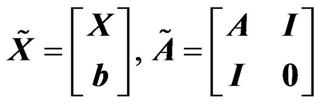 .
.
The vector  has a singular multivariate normal distribution with mean vector and covariance matrix
 respectively. For a random vector
  which has the general multivariate normal distribution
 standard results are that the cumulants of the quadratic form
  are
are
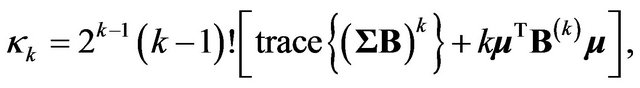
where 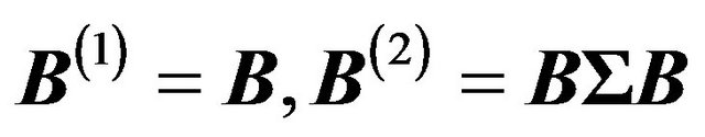 and so on, and that
 .
.
Substitution of ,
,  ,
, and
and  gives the results of Proposition 2.
B—Proof of Proposition 8
The return on the market portfolio is
 , where
  and
and  have the multivariate normal distribution
  as defined in Section 3. Conditional on
 , the expected value of
  is
is
The first term is the ratio of two variables which have a bivariate normal distribution. Cedilnik, Košmelj and Blejec [31] show that such a variable does not have an expected value or higher moments. This is sufficient to ensure that the unconditional moments of  are undefined.
C—Forecast Mean Vector and Covariance Matrix
Table A1. Forecast Mean Weekly Returns for 13 FTSE Indices.
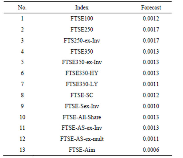
Table A2. Sample Covariance/Correlation Matrix.
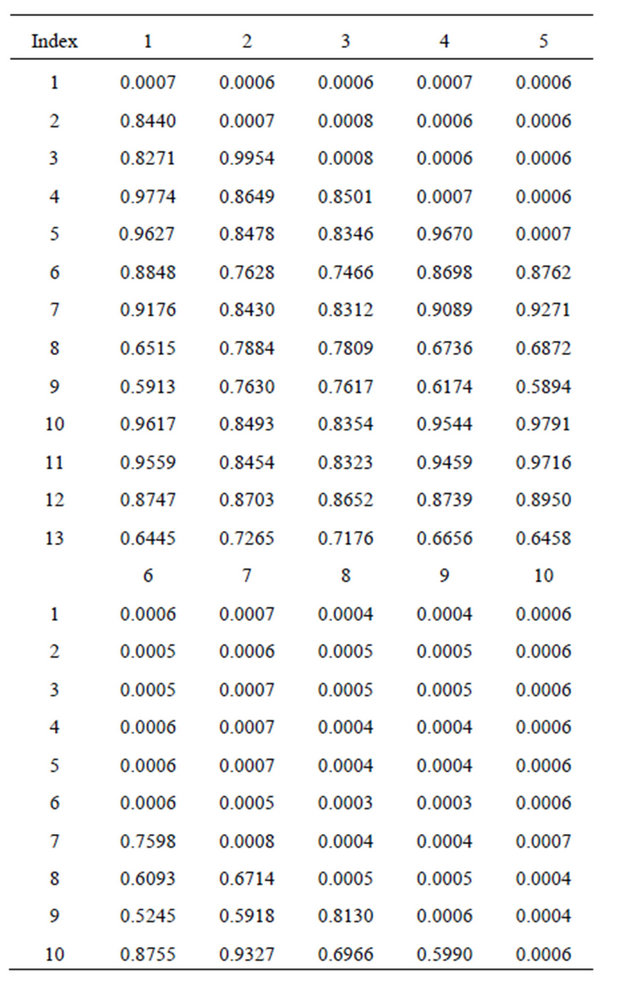
Continued
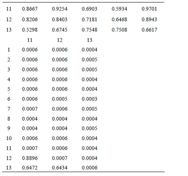
Correlations are shown below the leading diagonal.