ABSTRACT

We consider general regime switching stochastic volatility models where both the asset and the volatility dynamics depend on the values of a Markov jump process. Due to the stochastic volatility and the Markov regime switching, this financial market is thus incomplete and perfect pricing and hedging of options are not possible. Thus, we are interested in finding formulae to solve the problem of pricing and hedging options in this framework. For this, we use the local risk minimization approach to obtain pricing and hedging formulae based on solving a system of partial differential equations. Then we get also formulae to price volatility and variance swap options on these general regime switching stochastic volatility models.

1. Introduction

In this paper, we consider general regime switching stochastic volatility models where both the asset and the volatility dynamics depend on the values of a Markov jump process. We are interested in finding formulae to solve the problem of pricing and hedging contingent claims in this framework. However, due to the stochastic volatility and the Markov regime switching, the market is incomplete and thus perfect pricing and hedging are not possible. Hence, to hedge derivatives, we adopt firstly the local-risk minimization approach studied by Föllmer and Schweizer in [1]. This approach consists of controlling the hedging errors at each instant by minimizing the conditional variances of the instantaneous cost increments. Health et al. in [2], provided comparative theoretical and numerical results on risks, values and hedging strategies for this approach versus the meanvariance (see [3] or [4] for more details on this approach), in the specific case of stochastic volatility models. We propose in this paper to apply the local risk minimization approach to a more global class of stochastic volatility models since we will assume in the sequel that all parameters of the model depend on the values of a Markov jump process. Hence, we will work on a global class of regime switching stochastic volatility models. We will obtain formulae to give the price of contingent claims by solving a system of partial differential equations. We will also obtain the optimal strategy which solves the local risk minimization hedging problem.

There has been considerable interest in applications of regime switching models driven by a Markov process to various financial problems. Elliott et al. in [5] provided an overview of hidden Markov chain models. Indeed, the use of Markov switching in diffusions allows us to have different levels of drift or volatility during time. Moreover these regime switching activities are a better fit for economic times series data than non regime switching models and also allow us to better capture some market features or economics behaviors such as recession and financial crisis periods (see for example Goutte and Zou in [6]). Thus, Di Masi et al. in [7] considered the problem of hedging an European call option for a (nonstochastic volatility) diffusion models where the drift and volatility are functions of a Markov jump process.

Furthermore, we are also interested in pricing volatility derivatives, such as variance and volatility swaps. Broadie et al. in [8] studied the pricing and hedging of variance swaps and other volatility derivatives in the classical Heston stochastic volatility model introduced by Heston in [9]. Elliott et al. in [10] then developed a model for pricing the same class of derivatives but under a Markov-modulated version of this stochastic volatility model. In their paper, they only considered the case where not all the parameters of the model depend on the state of the Markov process. Moreover, they studied only the Heston stochastic volatility model. Hence, based on these two preceding works, we will extend this methodology to our global class of regime switching stochastic volatility models. Thus, we will obtain formulae to price options on the stochastic volatility process such as variance and volatility swaps.

This paper is arranged as follows: Section 1 gives the notion of the regime switching framework and presents our regime switching stochastic volatility models. Section 2 solves the problem of pricing and hedging using the local risk minimization approach. Section 3 then gives the formulas to price options on the volatility process.

2. The Stochastic Regime Switching Volatility Model

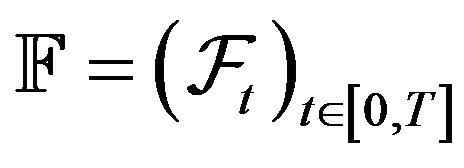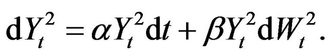
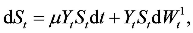
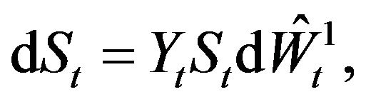
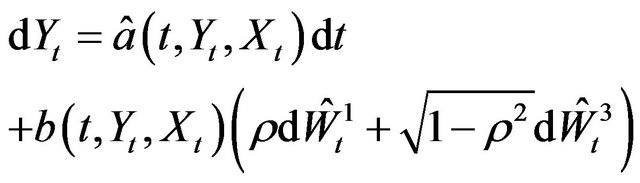
Let be a filtered probability space with filtration satisfying the usual conditions for some fixed but arbitrary time horizon. We consider a general stochastic volatility model defined by the stochastic differential equations:

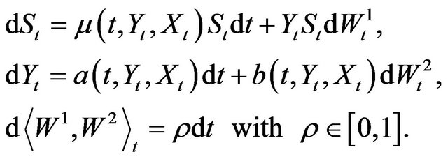(1.1)

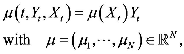
where and are two correlated Brownian motions. In fact, the process represents the discounted price process of a tradable asset price process

divided by a Bond price process. The process

represents the savings account in a riskless asset.

is a real stochastic process which is adapted and is a Markov jump process on finite state space. It can be viewed as an observable exogenous quantity. We assume that the time invariant matrix denotes the infinitesimal generator of, where is an infinitesimal intensity of. This generator is defined as, for all and for all.

Then, the semi-martingale decomposition for is given by

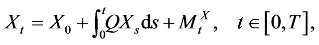
where is an -valued martingale with respect to, which is the natural filtration generated by the Markov process under.

Hence, in our model, there are three sources of randomness:, and. We will denote by

the filtration generated by the two Brownian motions. Finally, we will denote by the global filtration.

Let be the sequential jump times of (i.e.) and a jump measure of, i.e. the integer-valued random measure given by

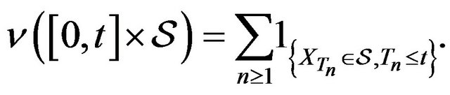(1.2)

Then the -compensator of is given by

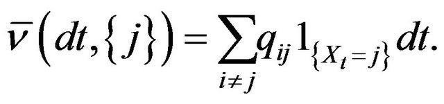(1.3)

Assumption 1.1

1) We assume all the hypothesis to ensure the existences and the regularities of the solutions of our model (1.1) (see for example [11] for more details). Hence, the system of stochastic differential Equations (1.1) admits a unique strong continuous solution for the vector process with a strictly positive price process and a volatility process.

2) We assume moreover that the Markov process is independent to both processes and.

Remark 1.1 This independence implies that the Markov process is an exogenous factor of the market information. Thus, it can be viewed as an exogenous factor such as an economic impact factor. An economic interpretation of this is that this Markov process can represent a credit rating of a firm. Indeed, assume that our stochastic volatility model describes the price of a commodity produced by the firm, then the Markov process can represent the credit rating of this firm given by an exogenous rating company as “Standard and Poors”. Thus, it is natural to think that the dynamic of the commodity’s price, produced by the firm, depends on the value of this notation.

To exclude arbitrage opportunities, we assume that the process S admits an equivalent local martingale measure (ELMM). In the sense that it is a probability measure with the same null sets as and such that the process S is a local martingale under. We will denote, in the sequel, by the set of all ELMMs.

Remark 1.2

1) We can rewrite the Brownian motion as , where the process is another Brownian motion such that processes and are now independent.

2) The condition that S should be a -local martingale fixes the effect of the Girsanov transformation of but allows us for different transformations on the independent Brownian motion defined in point 1. Consequently, if the correlation factor satisfies, then the set contains more than one element and so the financial market is then incomplete. Moreover, there is an other source of incompleteness of the market which is the dependence of processes and with respect to the Markov process.

We give now some examples of classical stochastic volatility models which are contained in our model (1.1).

Example 1.1 Hull-White:

Stein-Stein:

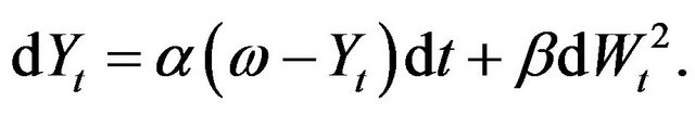
Heston:

3. Pricing and Hedging via Local Risk Minimization Approach

We are interested, in this section, in the hedging of an European contingent claims with an -measurable squared integrable random variable based on the dynamics given by (1.1). As an example of this payoff, we can take an European call option: with maturity T and strike K > 0.

We consider here the local risk-minimization approach to hedge in this incomplete market. We recall some definitions of this approach.

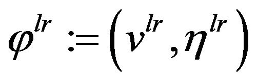
Definition 2.1 An hedging strategy is a pair 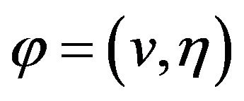such that is a predictable process which satisfies

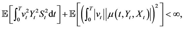(2.4)

and 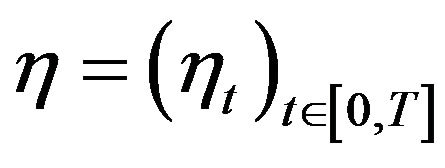is an adapted process such that

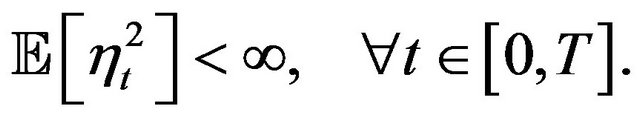(2.5)

We will denote by the set of strategies which satisfy (2.4) and (2.5).

The hedging strategy defines a portfolio where denotes the number of shares of the risky asset held by the investor at time and denotes the amount invested at time in the bond.

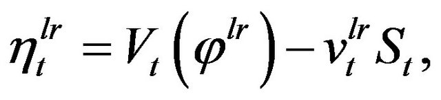
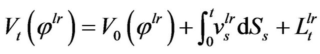
Definition 2.2 Given a hedging strategy, we call the Value process of this corresponding portfolio the right continuous process given by

(2.6)

Definition 2.3 Given a hedging strategy, we call the Cost process of this corresponding portfolio the process given by

(2.7)

We can see that the quantity represents the hedging gains or losses up to time following the hedging strategy. A hedging strategy is called self-financing if its cost process is -a.s. constant over the time and mean self-financing if is a -martingale. If is square integrable, then the risk process of is defined by

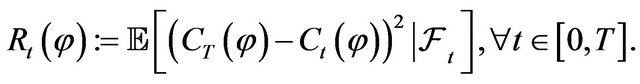(2.8)

Remark 2.3 Since the contingent claim is - measurable and is adapted, there always exists a hedging strategy such that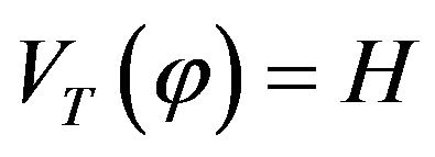. Indeed, we can take and for all.

3.1. Local Risk Minimization Approach

We only consider hedging strategies which replicate contingent claim at time. This means that we only allow hedging strategies such that

(2.9)

Thus, the hedging problem is so to find the strategy which minimizes at time the quadratic risk:

(2.10)

The idea is so to control the hedging errors at each instant by minimizing the conditional variances of the instantaneous cost increments sequentially over time.

Remark 2.4 An alternative approach to hedge in incomplete market is the mean-variance approach (see [3]). In fact, in this approach, the aim is to minimize the global risk over the entire time. Hence, it is a different approach than the local risk minimization which focuses on the minimization of the second moments of the infinitesimal cost increments (8).

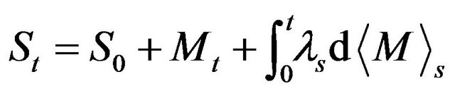
Therefore, the study of this minimization problem in a general semimartingale case is due to Schweizer [3] and it requires more assumptions on the asset dynamic. We assume firstly that can be decomposed as

where is a real valued locally squared integrable local -martingale null at zero and A is a real valued adapted continuous process of finite variation also null at zero.

We recall now the Definition of the Structure Condition (SC). We say that the process satisfies the (SC) if there exists a predictable process such that the process is absolutely continuous with respect to (i.e. the oblique bracket). In the sense that

and such that the so called mean variance tradeoff process (MVT) satisfies

Lemma 2.1 Since, we have that if the process is continuous then (SC) is satisfied.

Proof. See Theorem 1 of Schweizer [4].

Proposition 2.24 of Föllmer and Schweizer in [1] shows that finding a locally risk minimizing strategy for a given contingent claim is equivalent to finding a decomposition of of the form:

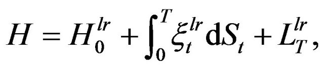(2.11)

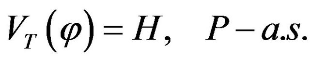
where is a constant, is a predictable process satisfying Condition (2.4) and is a square integrable -martingale null at 0 and strongly orthogonal to (i.e. is a P-martingale). The representation (2.11) is usually referred to as the Föllmer-Schweizer (FS) decomposition of the random variable. Once we have (2.11), then the desired hedging strategy, which is locally risk minimizing, is then given, for all, by

(2.12)

and

(2.13)

where

(2.14)

with

(2.15)

In view of these results, finding the Föllmer-Schweizer decomposition (2.11) of a given contingent claim is important because it allows us to obtain the locally risk minimizing strategy. Monat and Sticker in [12] and Pham et al. in [13] give sufficient conditions to prove the existence of this decomposition. We therefore explain how one can often obtain this decomposition by switching to a suitably chosen martingale measure for S. Indeed, as it is shown in [1] and [4], there exists a measure, which is the so called minimal equivalent local martingale measure (minimal ELMM), such that

(2.16)

where denotes the conditional expectation under.

Remark 2.5 If there exists a locally risk minimizing strategy, then we can use the expression of appearing in (2.16) as a price of the contingent claim at time.

In the case where the process is continuous (which is our case), Theorem 1 of [1] allows us to construct uniquely. Indeed, we have the following result:

Proposition 2.1 exists if and only if for all

(2.17)

is a square integrable martingale under.

Moreover, defines a probability measure equivalent to which is in since one easily verifies that is a local -martingale.

3.2. Markovian Regime Switching Case

Let, and given by the model (1.1), then the local risk minimizing hedging strategy can be obtained in two steps:

1) Determine and deduce the dynamic of under.

2) Find the Galtchouk-Kunita-Watanabe decomposition of with respect to under.

Then, the optimal local risk minimizing hedging strategy is given by (2.12) and (2.13).

3.2.1. Finding

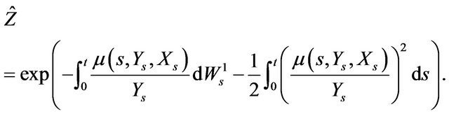
According to the previous subsection, the density process of the minimal ELMM with respect to is given by the Equation (2.17). We can firstly remark that

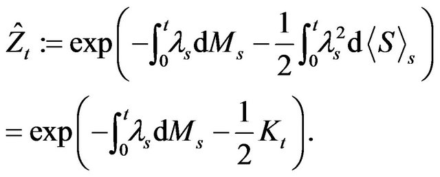
Since is continuous, we have first of all to determine the canonical decomposition

of the asset process under.

Proposition 2.2 Assume that the regime stochastic volatility model follows (1.1) then we have, for all, that

therefore we obtain

Proof. It comes immediately from the definition of the dynamic of our model (1.1).

We are now able to determine the dynamic of our model under.

Proposition 2.3 Assume that is a true -martingale, then the dynamic of the model (1.1) under is given for all by

(2.18)

with

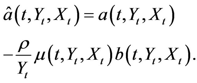(2.19)

Proof. Since is a -martingale, Girsanov’s theorem implies that 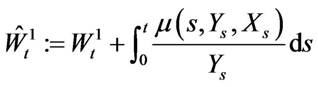and

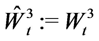are independent -Brownian motions. Hence

and

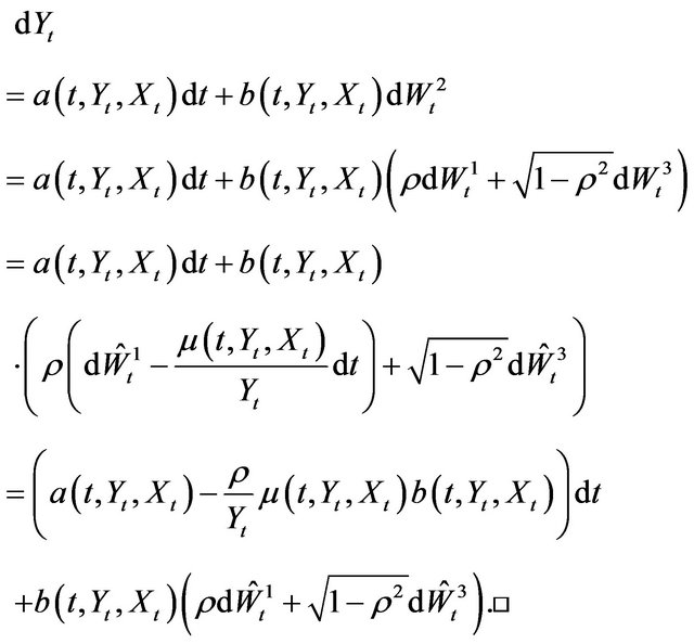
3.2.2. Decomposition of the Contingent Claim with Respect to under

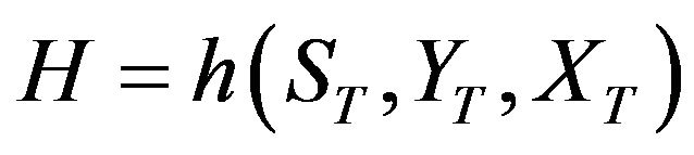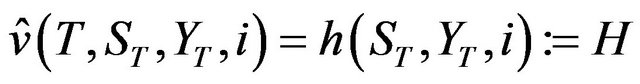
Let be a contingent claim of the form , then finding the Galtchouk-KunitaWatanabe decomposition of under reduces to solve a system of partial differential equations if one exploits the Markovian structure. Indeed, using the Markov property, we can rewrite (2.16):

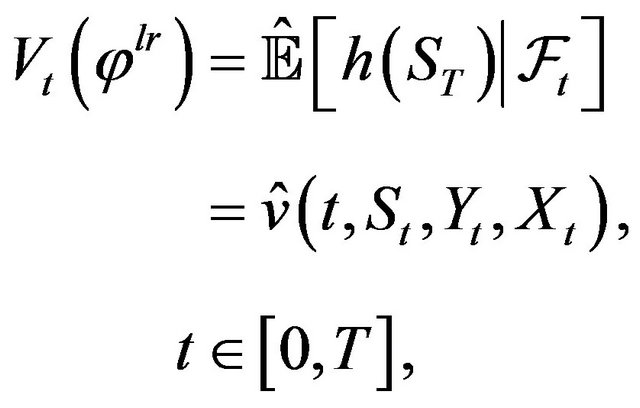
for some function defined on.

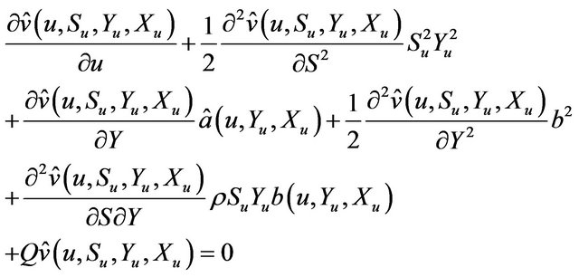
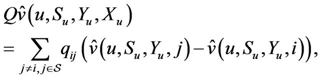
Proposition 2.4 For all, if, then is the solution to the system of partial differential equations given by

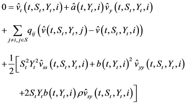(2.20)

with terminal condition for all given by

and where,

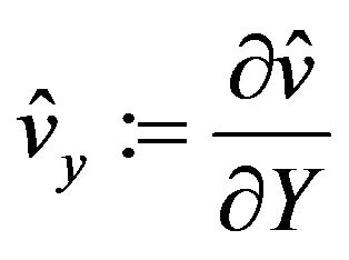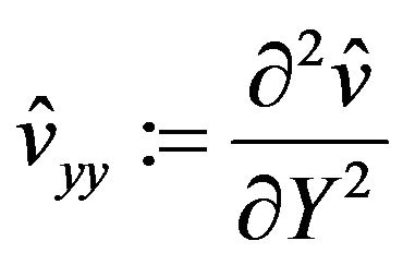, , and.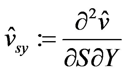

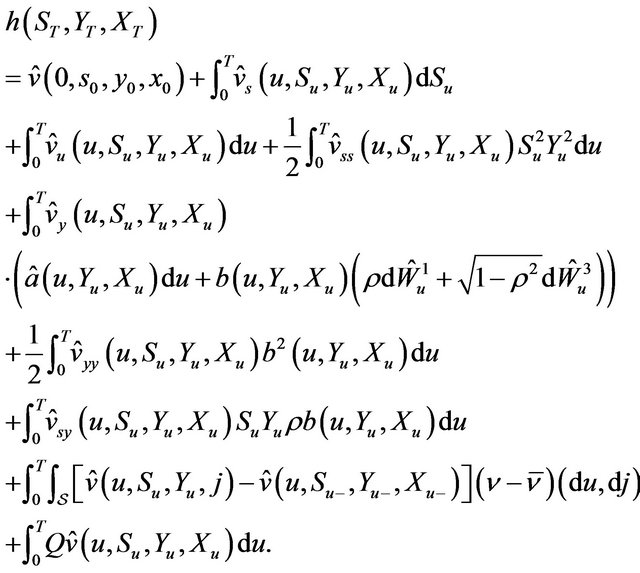
Proof. Since

(2.21)

and notice that for any function on , which is right continuous and with left limits in, we have

Hence, replacing the last equality in (2.21) gives

The function is a -martingale so all boundary terms are null. Hence we obtain that need to satisfy

with terminal condition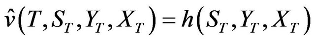. Moreover,

where 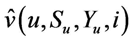means that at time the Markov process is in state (i.e.). Hence with, we obtain the expected result.□

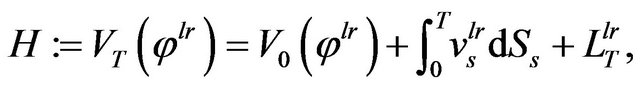
Example 2.2 (Pricing European call options on the underlying process S) The value of an European call option on the stock price with maturity T and strike K is given by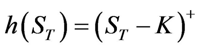. Hence we can apply Proposition 2.4 with

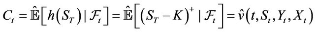
where the terminal conditions for all are given by.

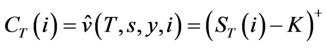According to (2.12) and (2.15), we are now able to find the decomposition of with respect to under and so the locally risk minimizing -admissible strategy.

Theorem 2.1 For all, we have that the locally risk-minimizing hedging strategy of, is given by

(2.22)

(2.23)

where

and

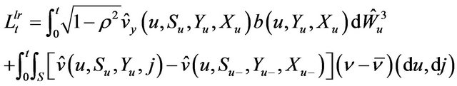
Remark 2.6 Moreover, taking the problem at time, we get

which is the so-called Föllmer-Schweizer decomposition of the random variable.

Proof. Let, apply Ito’s formula to 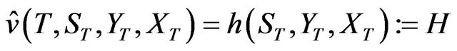, then by (2.21), we obtain:

We apply now the result of Proposition 2.4 to obtain

Combining this result with

gives the expected result.□

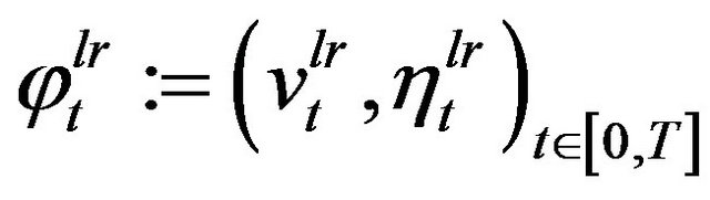
We can also obtain a formulation of the conditional expected squared cost on the time interval for the locally risk-minimizing strategy.

Proposition 2.5 We have, for all, that the conditional expected squared cost on the interval for the locally risk-minimizing strategy is given by

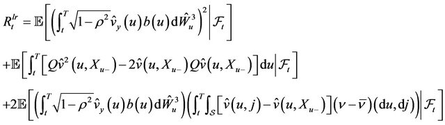
Proof. Applying the result of Theorem 2.1 in (2.8) we obtain

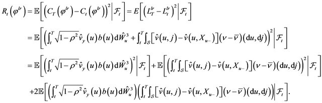
We can also simplify the second expectation

To apply all the results about local risk minimizing hedging strategy , it remains to prove that is a true P-martingale and square integrable under P. A wellknown sufficient condition for both is the boundedness of the mean variance tradeoff process, stated in Proposition 0.2, uniformly in and (see [12-14]).

Proposition 2.6 If the mean variance tradeoff process, defined in Proposition 0.2, is uniformly bounded in and then we have that:

1) is a true -martingale and square integrable under.

2) H admits a Föllmer-Schweizer decomposition given by (2.11).

3), defined in (2.12) and (2.13), is the local risk minimizing hedging strategy.

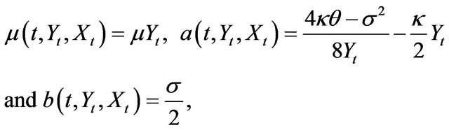
Example 2.3 (Heston model) We can take for the model (1.1) a Heston model case. Hence, by Example 1.1, we take

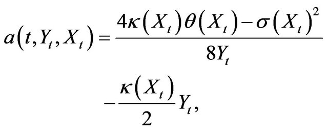
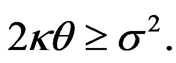
The constants, and are all nonnegative for all. And we assume for the existence and positivity of the solution that for all,

.

The model is then given by

and the corresponding mean variance tradeoff process is then given by

Hence the MVT process K is deterministic so bounded uniformly in and. This implies that is a P-martingale and so that we can apply all the results mentioned before.

4. Pricing Option on the Volatility:

We are now interested in establishing some formulae to price options based on the stochastic volatility process.

4.1. Variance Swap

A variance swap is a forward contract on the annualized variance, which is the square of the realized annual volatility. Thus, let 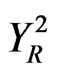denote the realized annual stock variance over the life of the contract. Then it is given by:

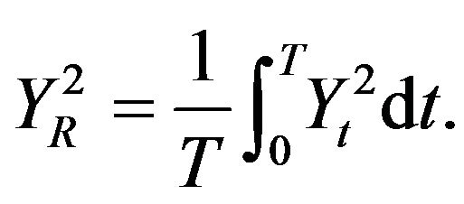(3.24)

Let and denote the delivery price for variance and the notional amount of the swap in dollars per annualized volatility point squared. Then, the payoff of the variance swap at the maturity time is given by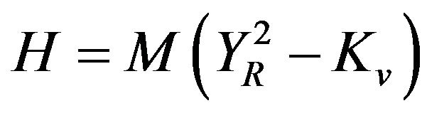. Intuitively, the buyer will receive dollars for each point by which the realized annual variance has exceeded the variance delivery price. The results provided, in the sequel, are an extension of the results obtained in [10]. Indeed, firstly we study more general class of stochastic volatility models and secondly we apply our results, in the particular case of Heston model, but where not only the long-term volatility level depends on the regime but also the speed of mean reversion on the volatility of the volatility.

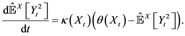
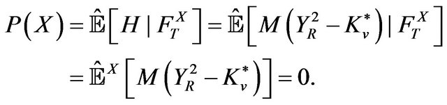
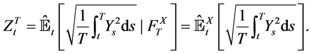
Hence, we start by considering the evaluation of the conditional price of a derivative H given the information about the sample path of the Markov process from time 0 to time T (i.e.). This means that we assume to know all the historical path of the Markov process. Assume, also, that we are under the minimal ELMM. Thus, we recall that in this case our regime switching model is given by:

with

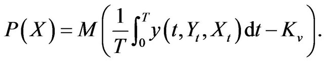
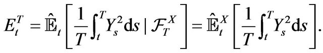
. In particular, given, the conditional price of the variance swap is given by

(3.25)

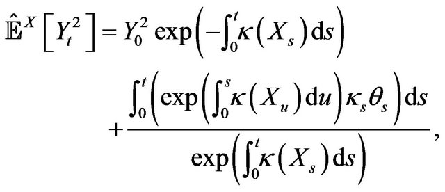
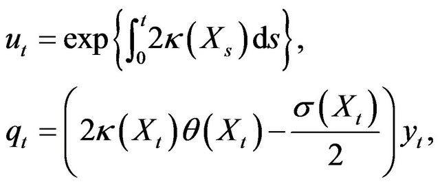
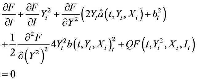
Hence, if we denote as previous

, we obtain by Itô formula that for all,

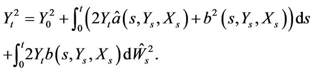(3.26)

Thus, given, we get

(3.27)

So

(3.28)

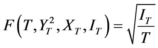
Assumption 3.2 Assume that we know the solution of Equation (3.28) which we will denote by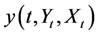, for all.

Proposition 3.7 Under Assumption 3.2, we have, for all, that the conditional variance swap price P(X) is given by

(3.29)

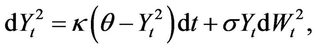
Example 3.4 (Heston Model) Assume that we are in the Heston model case. Hence as mentioned in Example 1.1 we take

and

Then the dynamic of is given by

.

Moreover, (3.28) becomes

Let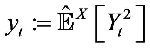, then we have to solve the differential equation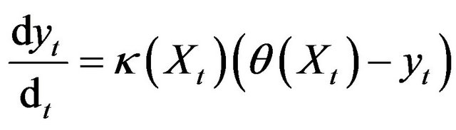. The solution of this differential equation is given for all by

Thus, we get

(3.30)

We can now obtain the conditional variance swap price by applying Proposition 3.7:

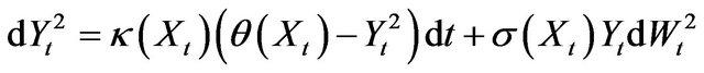
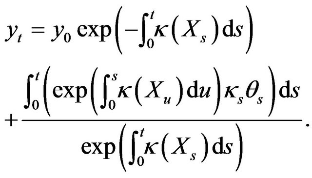
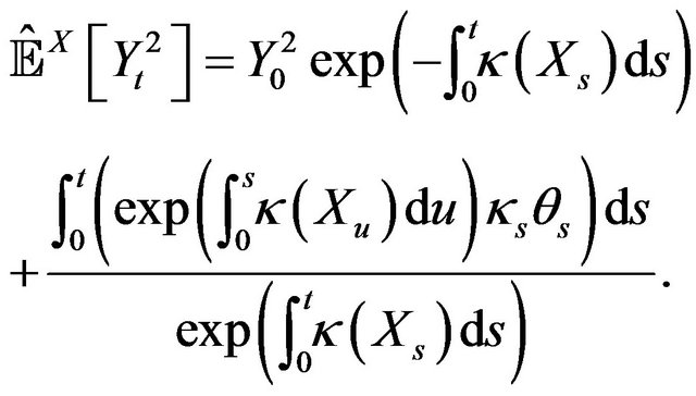
We can also obtain the value of the conditional variance given the full history of.

Lemma 3.2 For all, the conditional variance of is given by

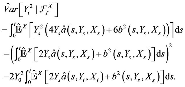
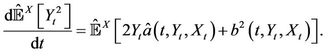
Proof. By Ito’s lemma we get

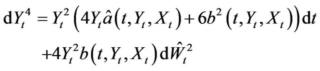
Hence, given, we find that

(3.31)

Using (3.27) and the definition of the variance give the result.

Example 3.5 (Heston Model) We continue the study of the Heston model case (see Example 3.4). Thus Equation (3.31) gives

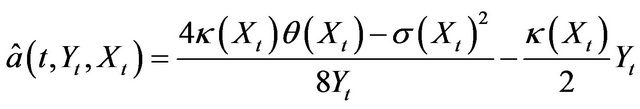
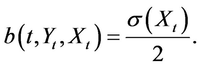
Given (3.30), we know that

which is a function of time and the Markov process. Let, then we have to solve the differential equation given by

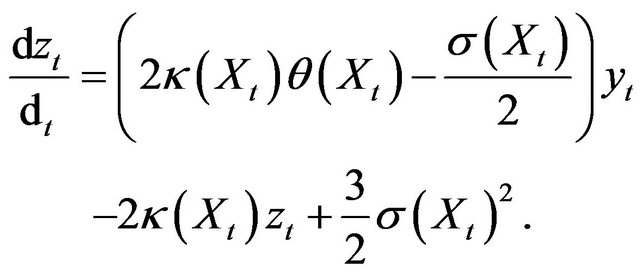
The solution of this differential equation is given for all by

where

We finally obtain in the Heston model case that

and that the conditional variance is equal to

4.2. Pricing Volatility Swaps

In this section, we follow the same methodology studied by Broadie and Jain in [8] where there is no regime switching component. We recall that the realized annual stock variance over the life of the contract is given by (3.24) and depends on the values of the Markov process

. Denote by 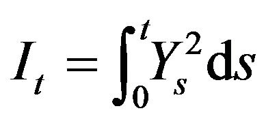the accumulated variance between time 0 to. We recall that the process is the solution of the stochastic differential equation given by

Hence is the solution of the stochastic differential equation given by. Let define by the expectation at time with respect to

(3.32)

Hence 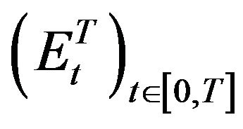depends on the variance process

of the underlying asset and on the Markov process. We call by fair conditional variance strike price the quantity which is defined such that Equation 3.25 vanishes:

Then, we have that 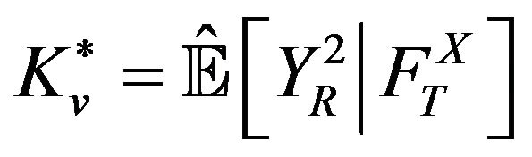and for time

, we obtain that. We define now the forward price process as

(3.33)

Proposition 3.8 The forward price process can be expressed as a function 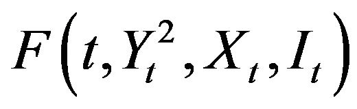and it is the solution of the system of stochastic differential equations given by

(3.34)

with boundary condition given by

.

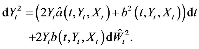
Proof. Rewrite as

.

Applying Itô Lemma to, using (3.26) and the fact that the forward price measure is a martingale give the expected result.

5. Conclusions

In this paper, we studied the problem of pricing and hedging options based on an asset which is modeled by a regime switching stochastic volatility model. We presented firstly this class of regime switching stochastic volatility models. We shown that this class of regime switching models encompasses a large panel of classical financial models. We also explained the interest in applications of this kind of models. Secondly, we used the local risk minimization approach to solve the problem of pricing and hedging contingent claims in this incomplete market. Thus, we obtained pricing and hedging formulae and also the formula of the optimal hedging strategy. Finally, we fund formulae to price volatility and variance swap options by solving a system of stochastic differential equations.

Some possible future directions in this field of research are the following:

-     Develop a method to estimate all the parameters of this class of regime switching models, including the hidden Markov chain (its transition matrix);

-     Apply these pricing and hedging formulae to economic and financial data. Indeed, regarding the existing literature, a good candidate could be the electricity spot price;

-     Construct a method to evaluate quickly the solutions of the system of stochastic differential Equations (2.20) and (3.34). A system of spatial and time discretization grids could be considered and investigated.

REFERENCES

- H. Föllmer and M. Schweizer, “Hedging Contingent Claims under Incomplete Information,” In: M. H. A. Davis and R. J. Elliott, Eds., Applied Stochastic Analysis, Stochastics Monographes, Gordon and Breach, 1991, 389-414.
- D. Health, E. Platen and M. Schweizer, “A Comparison of Two Quadratic Approaches to Hedging in Incomplete Markets,” MATHEMATICAL Finance, Vol. 11, No. 4, 2001, pp. 385-413. doi:10.1111/1467-9965.00122
- M. Schweizer, “Option Hedging for Semimartingales,” Stochastic Processes and Their Applications, Vol. 37, No. 2, 1991, pp. 339-363. doi:10.1016/0304-4149(91)90053-F
- M. Schweizer, “On the Minimal Martingale Measure and the Föllmer-Schweizer Decomposition,” Stochastic Analysis and Applications, Vol. 13, No. 5, 1995, pp. 573-599. doi:10.1080/07362999508809418
- R. J. Elliott, L. Aggoun and J. B. Moore, “Hidden Markov Models: Estimation and Control,” Springer-Verlag, New York.
- S. Goutte and B. Zou, “Continuous Time Regime Switching Model Applied to Foreign Exchange Rate,” CREA Discussion Paper Series 11-16, Center for Research in Economic Analysis, University of Luxembourg, Luxembourg City, 2012.
- G. B. Di Masi, Yu. M. Kabanov and W. J. Runggaldier, “Mean Variance Hedging of Options on Stocks with Markov Volatilities,” Theory of Probability and Its Applications, Vol. 39, No. 1. 1994, pp. 172-182. doi:10.1137/1139008
- M. Broadie and A. Jain, “Pricing and Hedging Volatility Derivatives,” Journal of Derivatives, Vol. 15, No. 3, 2008, pp. 7-24. doi:10.3905/jod.2008.702503
- S. L. Heston, “A Closed-Form Solution for Options with Stochastic with Applications to Bond and Currency Options,” Review of Financial Studies, Vol. 6, No. 2, 1993, pp. 237-343. doi:10.1093/rfs/6.2.327
- R. J. Elliott, T. K. Siu, L. Chan and J. W. Lau, “Pricing Volatility Swaps Under Heston’s Stochastic Volatility Model with Regime Switching,” Applied Mathematical Finance, Vol. 14, No. 1, 2006, pp. 41-62. doi:10.1080/13504860600659222
- M. Romano and N. Touzi, “Contingent Claims and Market Completeness in a Stochastic Volatility Model,” Mathematical Finance, Vol. 7, No. 4, 1997, pp. 399-410. doi:10.1111/1467-9965.00038
- P. Monat and C. Stricker, “Föllmer Schweizer Decomposition and Mean-Variance Hedging of General Claims,” Annals of Probability, Vol. 23, No. 2, 1995, pp. 605-628. doi:10.1214/aop/1176988281
- H. Pham, T. Rheinländer and M. Schweizer, “Mean-Variance Hedging for Continuous Processes: New Results and Examples,” Finance and Stochastics, Vol. 2, No. 2, 1998, pp. 173-198. doi:10.1007/s007800050037
- D. Lepingle and J. Mémin, “Sur l’Intégrabilité Uniforme des Martingales Exponentielles,” Zeitschrift für Wahrscheinlichkeitstheorie und verwandte Gebiete, Vol. 42, 1978, pp. 175-203.