Journal of Mathematical Finance
Vol.2 No.3(2012), Article ID:22133,13 pages DOI:10.4236/jmf.2012.23028
Do Idiosyncratic Risks in Multi-Factor Asset Pricing Models Really Contain a Hidden Non-Diversifiable Factor? A Diagnostic Testing Approach
1School of Business and Management, Azusa Pacific University, Azusa, USA
2College of Business, James Madison University, Harrisonburg, USA
Email: jjeng@apu.edu, liuqx@jmu.edu
Received May 25, 2012; revised June 28, 2012; accepted July 8, 2012
Keywords: Non-Diversifiable Factors; Rescaled Variance Test; Multifactor Pricing Models
ABSTRACT
This paper employs a new approach to analyze potentially omitted non-diversifiable factors in the idiosyncratic risks from multi-factor asset pricing models. It is shown that if there is an omitted non-diversifiable hidden factor, the idiosyncratic risks will contain persistent cross-sectional memory. An extended Rescaled Variance test generalized from L. Giraitis, P. Kokoszaka, R. Leipus, and G. Teyssiere [1] with finite forecast horizon is provided to investigate the cross-sectional memory of forecast errors in multifactor pricing models. Under the null hypothesis that idiosyncratic risks contain only short memory when there is no hidden non-diversifiable factor, we demonstrate that the extendedT-sample Rescaled Variance test statistic approximates a functional of weighted Brownian Bridge, which is distributed asymptotically as the T-sample Watson’s statistic presented by Maag [2]. Using this approach, our empirical tests that compare forecast errors from the CAPM and Fama-French [3] model with the excess returns of 1391 firms indicate that there is a strong likelihood that the CAPM may require further identification of hidden non-diversifiable factor(s). Yet, there lacks convincing evidence that the Fama-French [3] model has an omitted non-diversifiable factor in idiosyncratic risks.
1. Introduction
Empirical studies on asset pricing models generally require the application of some ad hoc information sets of proxies or reference variables. Since the genuine factor structures are unobservable for the specification of risk premia, the set of proxies or reference variables only represents the incomplete information set in a presumed factor structure for risk premium. In empirical studies, it is possible that the disturbance term of a presumed factor structure includes omitted factors in the process of projecting excess returns on an ad hoc information set. Numerous empirical studies, such as Goyal and Santa-Clara [4], Mayers [5], and Malkiel and Xu [6], show that the idiosyncratic risk volatility on a presumed factor structure or asset-pricing model may contain useful information in forecasting the stock returns. In a follow-up study to Goyal and Santa-Clara [4], Guo and Savickas [7] argue that the predictive power of idiosyncratic volatility goes down if consumption-wealth ratio is controlled for in the forecasting equation. T. Bali, N. Cakici, X. Yan and Z. Zhang [8] also shows that the finding of Goyal and Santa-Clara [4] is partially due to liquidity premium and small stocks traded in NASDAQ. With extended samples of stock returns, Balie [8] does not find any significant relation between equally weighted average stock volatileity and the value-weighted portfolio returns. A. Ang, R. J. Hodrick, Y. Xing, and X. Zhang [9], however, find that stocks with high idiosyncratic volatility (relative to the Fama and French [3] model) have low average returns pointing to a negative relation between idiosyncratic risks and stock returns. Fu [10] argues that idiosyncratic volatilities are time-varying and the results in A. Ang, R. J. Hodrick, Y. Xing, and X. Zhang [9] are largely driven by the return reversal of a subset of small stocks with high idiosyncratic volatilities. He instead finds a significantly positive relation between the estimated conditional idiosyncratic volatilities and expected returns using EGARCH models. Guo and Savickas [11] show that idiosyncratic volatility has statistically significant predictive power for aggregate stock market returns, and that idiosyncratic volatility performs just as well as the book-to-market factor in explaining the cross section of stock returns. However, all these time series/cross-sectional empirical studies focus mainly on the finding of explanatory variables for the stock returns. An issue that needs further attention is the diversifiability of the identified factor(s). Given that the systematic risk/factor(s) is non-diversifiable in asset pricing models, verification of diversifiability on these presumed factor(s) should be provided in addition to the identification of explanatory variables. In brief, the detection of possible explanatory factor(s) for stock returns although essential, should be followed by a study on the diversifiability of the identified factor(s).
Hence, discussions on additional hidden factor(s) in the idiosyncratic risks from presumed asset pricing models raise the following questions: Do idiosyncratic risks on a presumed asset pricing model really contain an essential hidden non-diversifiable factor that should be applied to asset pricing models? If so how can we test it?
Chamberlain and Rothschild [12] show that if asset returns have a k-factor approximate factor structure where k < n, and n is the number of assets then, the first k eigenvalues of the variance-covariance matrix of asset returns will be unbounded while the k + 1 eigenvalue of the matrix will be finite, as n grows to infinity. However, in empirical studies of asset returns, for any finite sample collected, eigenvalues of the variance-covariance matrix of asset returns under presumed factor structure are all finite. Verification on the growth of eigenvalues of these matrices across increasing sample sizes of asset returns is needed in empirical studies since the claim of approximate factor structure of Chamberlain and Rothschild [12] is based on an infinite dimensional setting. This paper provides an alternative test based on the fact that if the factor loadings of a hidden factor (in idiosyncratic risks) are non-diversifiable with respect to all well-diversified portfolios, a persistent cross-sectional memory among idiosyncratic risks will result. Specifically, if the asset returns follow the approximate factor structure with k + 1 factors where the fitted model is only equipped with k identified factors, then the (k + 1)-th eigenvalue of the variance-covariance matrix for asset returns (due to the hidden non-diversifiable factor loadings) will be unbounded, according to Chamberlain and Rothschild [12]. However, this property of unbounded non-diversifiable factor loadings can be shown to lead to a persistent crosssectional memory among the presumed idiosyncratic risks. Instead of applying eigenvalues or statistical procedures such as principal component analysis to examine the factor structure, the verification of the persistence of cross-sectional dependence among idiosyncratic risks becomes a diagnostic tool for asset pricing models and/or hidden factor(s). Many empirical studies show that idiosyncratic risk for asset pricing models is essential in pricing the asset returns. However, the verification for idiosyncratic risks as systematic/non-diversifiable factor(s) is still required for further studies. Specifically, if idiosyncratic risks or proxies of their volatility are indeed the common non-diversifiable factors among all asset returns, then they should appear as consistent components with persistent cross-sectional dependence in presumed asset pricing models. Although it may seem optimistic for empiricists to consider idiosyncratic risks as hidden factors when cross-sectional dependence or shortrun time-series predictability is discovered, these findings may not necessarily guarantee a non-diversifiable factor required for asset pricing models, unless further study is provided to verify that the identified factor or proxy is non-diversifiable.
The method developed in this study can verify the existence of a non-diversifiable hidden factor by testing if the error terms of asset pricing models are subject to a cross-sectional long dependence. Intuitively, under linear factor structure of excess returns, if there is a hidden non-diversifiable factor in idiosyncratic risks, then none of the weighted combinations of asset returns in the well-diversified portfolios will eliminate this factor. Specifically, the weighted sums of factor loadings for this hidden factor will not converge to zero asymptotically when the number of assets expands. Similar to time series setting, this property is closely related to the definition of cross-sectional long memory as the sums of cross-sectional covariances of these idiosyncratic risks will expand to infinity asymptotically. Therefore, the cross-sectional memory condition of idiosyncratic risk becomes a necessary condition, and thus an alternative test for the existence of non-diversifiable hidden factor.
Our diagnostic test provides an effective way to determine whether the factors found in these studies are transitory or persistent in cross-sectional memory, and thus to ascertain the validity of their findings. In other words, the verification of factor structure is reduced to the verification of persistence of cross-sectional dependence (for idiosyncratic risks) among these asset returns. Specifically, a forecast-error-based extended Rescaled Variance test is introduced here as an alternative statisticcal inference for idiosyncratic risk. Although long memory or long dependence has been discussed in many time series studies, the extension can be provided in random fields or set-indexed data such as Lavancier [13]. On the other hand, re-stacking and exchanging the time series horizon and cross-sectional indices as in White [14] for panel data, the asymptotic arguments on long memory time series can also be applied to the cross-sectional long dependence. The rest of this paper is organized as follows. Section 2 shows the model and a theorem for the long-memory properties of idiosyncratic risks where their partial sums of cross-sectional co-variances grow to infinity asymptotically if the omitted factor is non-diversifiable. The proofs of these arguments are shown in the appendix. Section 3 shows the modified T-sample Rescaled Variance Test when given with finite-timehorizon panel data. Section 4 shows applications and empirical findings of the test in detecting the omitted non-diversifiable factor on idiosyncratic risks of FamaFrench [3] model for 1391 excess returns, followed by the conclusion.
2. The Model
To derive the test, we first introduce a few prerequisites. Definition D1 describes a Hilbert space of real squaredintegrable random variables defined on the probability space1. The excess returns of assets forms a subset of this Hilbert space. Assumption A1 shows the conditions of factors or pre-specified reference variables applied as factors. The assumption allows different choice sets of instrumental or reference variables applied to specify the risk premium. These choice sets may be evolving over time or different sample sizes. In particular, the reference variables may be generated by the innovations from the multivariate time series models of pre-specified economic variables in a conditional expectation approach. Assumption A2 is to describe the presumed multi-factor model of the asset returns. Assumption A3 shows the possible missing factor and idiosyncratic risk in the excess return after projecting on the presumed explanatory variables. Assumption A4 provides a condition for diversification of the genuine noises in pricing models.
Definition D1: Let  be a Hilbert space of squared-integrable (with respect to probability measure P) real-valued random variables on complete probability space
  where H is endowed with the
  -norm
-norm |, where
  for
for .
.
Let the inner product of H be denoted as  for all
 . In addition,
  represents a sequence of all assets’ excess returns contained in H.
| 3As this studyfocuses on the identification of hidden non-diversifiable factors, the possibly time-varying risk premium is left for future studies. |
Assumption A1: Let 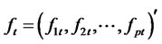 be a vector of p orthogonal perceived factors2 (defined in H) at time t for the multi-factor pricing model,
  is the j-th factor at time t. Or, in particular,
  s are orthogonal reference variables from the available information set for the asset-pricingfactors. In addition,
  , where
 for all
 .
.
Assumption A2: Let the excess return  for each asset i at time t be expressed in the fitted factor structure as
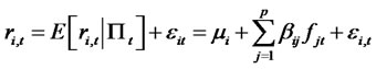 , (1)
, (1)
where  as randomly assigned subindices for the asset returns, and
 , where
  represents the information filtration (including lagged dependent variables) up to time t,
  stands for the conditional expected excess return
  3,
3, 
stands for the projection error (or so-called “presumed” idiosyncratic risk) for asset i and time t with the assumed multifactor pricing model.
Assumption A3: Let the projection error or presumed idiosyncratic risk (if contains a hidden factor) be expressed as,  , where
  represents a stationary stochastic hidden factor with a non-degenerated distribution,
  ,
,  , such that
  is orthogonal to all pre-selected factors as
 , and
, and  is cross-sectional stationary for all assets and inter-temporal independent over time. The
  represents the non-stochastic unobservable factor loading for asset i on the hidden factor
  for all i’s,
  The
The  is a cross-sectional mean-zero stationary random noise with finite moments and is independent of
 ,
,
 .
.
Also, let
such that all sequences of  belong to the factor-loading space
  with
with  -norm.
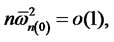
Assumption A3 imposes an asymptotic condition for the absolute factor loading(s) on the hidden factor. This is to ensure that as the size of portfolio expands, the factor loadings won’t be exploding—provided that the excess returns are in the Hilbert space H. To apply the ideas of diversification, a few definitions on the feasible weights in the factor pricing models are introduced in the followings. Definition D2 and D3 are to formulate the diversification in an infinite dimensional quadratic functional to define the opportunity set for sequence of feasible weights applied to each asset. The definition of non-diversifiable hidden factor is provided in D4. The notation  represents the numbers of assets n grows sufficiently large asymptotically. Specifically, the limit of weighted sums of hidden factor loadings
 is denoted as
  and the limit of weights
  as
as , respectively.
Definition D2: Let W be a compact sub-space of  space endowed with the
  -norm that for any
 where W consists of all real bounded sequences of nondegenerated diversifying feasible weights
  such that
  and
and , where
  contains sequences of
  with only finitely many numbers of non-zero weights that for each
 and W* is the closed subset of W with
  4,
4,  and
and ,
,
| 6It is easy to show that the diversification problem also focuses on the variances and co-variances of |
 where the idiosyncratic risk has been diversified away. The functional
  will be
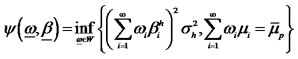 , where
  is the 2nd-order moment of the hidden factor. In addition, we confine the weights to lie in
  space so that the weights are subject to appropriate normalization.
 where  stands for the mean return for asset i,
  is the mean rate of return for the portfolio5. Let
  =
= ,
,  ,
,  is an infinite dimensional closed sub-space of
  -space for bounded sequences of factor-loading
endowed with the  -norm as
 .
.
Definition D3: Let  be a weakly lower semi-continuous diversification functional, where
 for a given
  in
in . The diversification problem of the portfolio is defined as
 where W* is the closed subset of W as defined in Definition D2.
Given the above definition, the idea of diversifiable factor rests on the opportunity set of the infinite dimensional optimization problem. For the non-diversifiable factor, its hidden factor loadings can’t be eliminated by any possible sequence of feasible diversifying weights in W* as .
.
Definition D4: The hidden factor  for all the factor-loading sequences such that
 where
where , is denoted as W*-diversifiable with increasing numbers of assets if and only if
for all , and the hidden factor is denoted as nondiversifiable in W* when
  for all
 as
as . That is, the hidden factor is W*-non-diversifiable, if and only if all sequences of diversifying weights will not drive the weighted sums of factor loadings to zero6.
Assumption A4 (Diversification of random noises):
the weighted sum as  almost surely for all
 as
as .
.
With the above framework, we can now show that diversification of the hidden factor depends on the crosssectional memory conditions (or intensity of memory) of hidden factor. This in turns provides us with statistical hypotheses to test the existence of non-diversifiable hidden factor.
Theorem 1.1: If for any date t, there exists a non-diversifiable stationary hidden factor in idiosyncratic risk 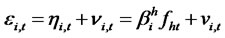 and let the distance function between indices of asset returns with arbitrary orders (denoted as s and i respectively) be defined as
  for
for , and the cross-sectional covariance function be defined as
 the presumed idiosyncratic risk
  is a crosssectional perturbed long-dependent series for any date t, such that
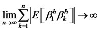
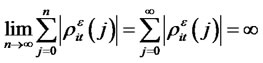 for all the presumed idiosyncratic risk
  as numbers of assets n grow. Conversely, if
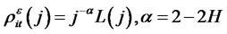
  is covariance-stationary and
  for all i’s and t’s, where L(j) is a slowly-varying function of j,
 ,
,  (i.e. the
  is a crosssectional long dependent series for any t), and for some sufficiently small
 , and for all
 7, (2)
 is a slowly-varying function of i that
 for
for 
then the hidden factor is non-diversifiable in W*.
Moreover, according to Zhou and Taqqu [15], a completely random re-ordering of samples will not impact the data’s long dependence. Consequently, when the cross-sectional sub-indices to asset returns are assigned randomly, like in many empirical studies, the cross-sectional long memory will not be influenced either. Hence, the diagnostic test on the memory condition of projection errors (or idiosyncratic risks) becomes an alternative method for identifying the non-diversifiable hidden factor.
3. Hypothesis Testing
In the following, we extend the framework of the Rescaled-Variance test of L. Giraitis, P. Kokoszaka, R. Leipus, and G. Teyssiere [1] with simultaneous inferences across finite forecast horizon to test the memory of idiosyncratic risks in fitted multifactor pricing models. The test statistics converge asymptotically to the T-sample Watson’s test statistic on unit circle where the asymptotic distribution is shown in Maag [2]. For the framework of analysis, we will assume that the time horizon is fixed. That is, the time horizon T for performing the test is finite while the numbers of cross-sectional observations n can be extended asymptotically as . A few definitions and assumptions are needed to establish the pre-requisites.
Definition D5: A random process  is called “self-similar”, if and only if
 , (3)
, (3)
where  is the Hurst exponent, the notation
stands for the equivalence of distributions. In addition, without loss of generality, we set the initial condition  almost surely. According to Embrechts and Maejima [16], for any self-similar process,
  if and only if
  almost surely. When
 , it implies that all autocorrelations of
  are equal to one.
Definition D6: Let  A mean-zero Gaussian process
  is called “fractional Brownian motion” if its auto-covariance function can be shown as
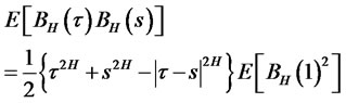 (4)
(4)
In particular, when , the process will have long-range dependence, when
 ,
,  will become the usual Brownian motion with independent identically distributed increments, if
 , the process is called “anti-persistent” with sum of auto-covariances being finite.
Assumption A5: Given Theorem 1.1 that for any date t,  in the pre-determined finite time horizon k of hypothesis testing, and for numbers of assets
 , where
 , and the hidden factor
is W*-non-diversifiable, and if  is covariance-stationary such that
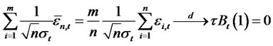
 and the long run variance
  of partial sum
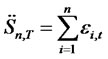
follows that
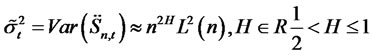
for  is a slowly-varying function of n such that
  for all
 , will converge in distribution as
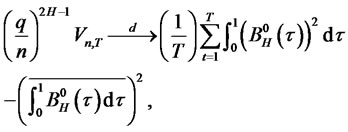
 (5)
(5)
where ,
,  ,
,  is the largest integer less than or equal to
 ,
,  is a fractional Brownian motion with Hurst exponent
 .
.
Assumption A6: Let the idiosyncratic risk  for any date t in the pre-determined finite time horizon T that may have a diversifiable hidden factor, contain only cross-sectional short memory as
 .
.
The sequence  satisfies the strong mixing condition such that the mixing coefficient
  as
as , where the mixing coefficient
 where the
  represents the
  -field generated by the set of random variables
  and
and  follows the invariance principle that as
 (6)
(6)
We hereby extend the Rescaled Variance statistic of L. Giraitis, P. Kokoszaka, R. Leipus, and G. Teyssiere [1] to a T-sample setting that analyzes the memory of the idiosyncratic risk with finite time horizon for panel data. Notice that the assumption A6 can be extended to include the (cross-sectional) heteroscedasticity in  and the following
  statistic converges to the same functional of Brownian bridges under the null hypothesis even though
  is not covariance-stationary. The conditions still holds under the non-stationary case as indicated by L. Giraitis, P. Kokoszaka, R. Leipus, and G. Teyssiere [1]. However, due to additional complexity that needs to be introduced, this is left for further studies.
Theorem 1.2: Given the above setting, for any date t,  , T is the finite time horizon for hypothesis testing, where
 , and
, and
 is the fourth order cumulant of cross-sectional covariance-stationary
  at date t then, under the null hypothesis that there is no non-diversifiable hidden factor in the idiosyncratic risk, for hypothesis testing with finite time horizon
 , the modified Rescaled Variance test is given as
 (7)
(7)
 (8)
(8)
 are T independent Brownian bridges where by definition,
 and the weights
 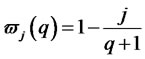 are the Bartlett weights such that
 ,
,  as
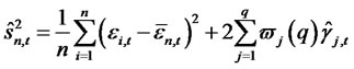
as  and the sample cross-sectional covariance function such as
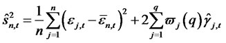
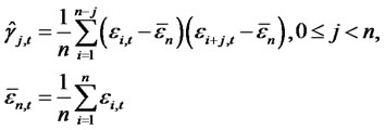
is the cross-sectional average,  are the error terms from the presumed asset pricing model for a given date t,
  stands for the largest integer that is less than or equal to the real number
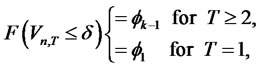
 , where the asymptotic distribution of
  (denoted as
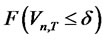 ) is shown by Maag [2] as
 (9)
(9)
 and
and  is the Hermite polynomial of order
  for argument z. Under the alternative hypothesis
  where
where  is cross-sectional covariance-stationary and there is a non-diversifiable factor in the idiosyncratic risk of presumed asset pricing model. In addition, for simplicity, let
 ,
, 
then,
 (10)
(10)
where  is the fractional Brownian Bridge with scaling parameter H. The test is also consistent that the statistic
  under the alternative hypothesis.
In other words, we reject the null hypothesis of short memory when  is large relative to the critical value chosen according to the significance level. When T is equal to one, the test is reduced to the Rescaled Variance test distributed as Watson’s test statistic. The reason that the test is referred to
  is that the test statistic converges to the same functional as Maag’s [2] statistic in testing identical distribution for all T groups without knowledge of the underlying cumulative distribution function for the data. The asymptotic distribution of such statistic is in turns, identical to the test statistic of
  groups under assumed cumulative distribution function according to Maag [2].
Notice that the above result is based on the genuine idiosyncratic risk . Yet, in the empirical studies, we can only observe either residuals or (out-ofsample) forecast errors from the fitted asset pricing models. Hence, we need to obtain the consistency of the sample statistics for any given (out-of-sample) forecast errors with cross-sectional observations
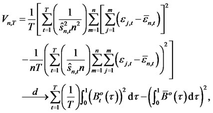
Theorem 1.3: Given that  for any date t in the finite time horizon T are the (cross-sectional) forecast errors for the presumed asset pricing model where the parameters for
 , are consistently estimated, and under the null hypothesis of no hidden non-diversifiable factor in
 , such that
when , the forecast error-based Rescaled Variance statistic is shown as
 , (11)
where
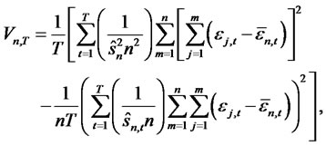
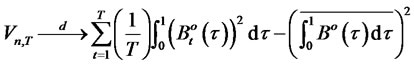
 (12)
(12)
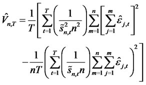 (13)
(13)
 is the estimate for
  by using
 , the forecast errors from the fitted asset pricing model.
4. Empirical Applications and Data
To test whether the idiosyncratic risks in Fama-French [3] model contain a hidden non-diversifiable factor or not, we collect the excess returns of 1391 randomly selected firms with different capitalizations and from different industries including agricultural products, chemical productions, financial, transportation, consumer goods, retail, entertainment, etc. These excess returns are collected from the firms in CRSP that have continuous monthly data in our sample period of January 1987 to December 2006. If there is a hidden non-diversifiable factor in idiosyncratic risks from Fama-French [3] model, finding of persistent memory in these idiosyncratic risks may provide the empirical evidence to verify the claim for its existence.
With regards to the possibility of survivorship bias in the CRSP data source, Li and Xu [17] argue that such survivorship bias is unlikely significant for the U.S. stock returns. In addition, Barber and Lyon [18] also show that the selection bias does not significantly affect the estimated factor premiums in equity returns of Fama-French [3] model, which implies that sample selection does not affect the empirical results of Fama-French [3] model. Hence, we select the explanatory variables for the regressions as those in the Fama-French [3] model as the asset pricing models of interest. And for comparison, we also apply our diagnostic test to the idiosyncratic risks from the CAPM. Furthermore, following the argument of Li and Mayer [19] that correction of dynamic selection bias does not improve the accuracy of forecasts of the model, the application with forecast errors from the fitted model seems more appropriate since our study is diagnostic for specifications in regressions. Therefore, we consider the out-of-sample forecast errors of both Fama-French [3] model and CAPM to test the null hypothesis that the hidden factor is diversifiable in the idiosyncratic risks.
Based on the tables and asymptotic cumulative distribution function provided by Maag’s [2], we select 24 months out-of-sample forecast errors (that is, T = 24) for the test period in verifying cross-sectional memory of idiosyncratic risks. The forecast errors for all these excess returns are obtained with the parameters estimated in the previous months of the in-sample period from January 1987 to December 2004, and are conditional on the updated explanatory variables in the asset pricing models applied here. The test period is from January 2005 to December 2006. The test statistics for different forecast horizons are calculated from T = 1 to T = 24 using the asymptotic cumulative distribution functions from Maag [2]. Notice that when T = 2, the test statistic actually conforms with Watson’s [19] two-sample test where its asymptotic distribution is identical to the statistic as in L. Giraitis, P. Kokoszaka, R. Leipus, and G. Teyssiere [1]. Hence, the asymptotic distributions applied to T = 2 and T = 1 are identical according to the asymptotic arguments in Maag [2] and Watson [20] as far as the two-sample tests are of concern, with an empirical application of Magg’s [2] tests shown in Brown [21].
Our extended Rescaled Variance  tests are performed under the null hypothesis that the hidden factor is diversifiable. The p-values of the statistics are calculated from the asymptotic cumulative distribution function provided by Maag [2]. Since the distribution function is not conventional, and that Maag’s [2] tabulation of critical values is limited to the case when maximum forecast horizon is T = 5, the
  statistics are considered as rejecting the null if the p-values are relatively smaller than the given 5% or 1% significance levels.
Table 1 presents the  test statistics and the corresponding p-values for testing the cross-sectional memory of idiosyncratic risks in the Fama-French [3] model. These test statistics are provided with different selections of q, which are denoted as the lags for possible crossNotes: The time index T stands for each month in the forecast horizon. For instance, T = 1 stands for January 2005, T = 2 stands for February 2005, and so forth. The table reports the test statistic with corresponding p-values denoted in parenthesis. If the p-value is less than the significance levels such as 5% or 1%, the null hypothesis that there is no non-diversifiable hidden factor is rejected.
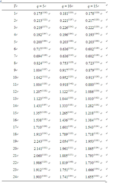
Table 1. T-sample rescaled variance tests on forecast errors of Fama-French (1993) Model.
sectional short-run memory in estimating long run variances of idiosyncratic risk under the null. For simplicity of exposition, we only report cases when q = 5, 10, 15, respectively.
For comparison purpose, we also perform the same diagnostic tests on the idiosyncratic risks from alternative models such as the CAPM, and the over-simplified case when excess returns are regressed only with a constant term. The test statistics are shown in Tables 2 and 3, respectively. All test statistics from these two alternative models reported in Tables 2 and 3 show that their p-values are all well below the 1% confidence level.
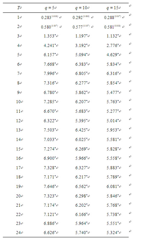
Table 2. T-sample rescaled variance tests on forecast errors of the CAPM.
Notes: Only the p-values of the first two months in forecast horizon are presented in parenthesis. Other p-values are replaced with an asterisk since they are much lower than 0.1%. The null hypothesis that there is no hidden non-diversifiable factor is rejected for all levels of T and q since all p-values are below 1% significance level.
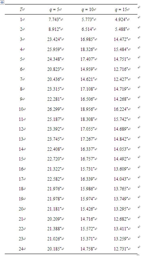
Table 3. T-sample rescaled variance tests on forecast errors when excess returns are regressed on a constant.
Notes: All p-values are replaced by an asterisk as they are much lower than 0.1%, and therefore the null hypothesis that there is no hidden non-diversifiable factor is rejected for all levels of T and q.
These statistics reject the null hypothesis that there is no hidden non-diversifiable factor in the idiosyncratic risks and suggest that there is a persistent cross-sectional memory in the idiosyncratic risks. In other words, these results imply that there is at least one hidden non-diversifiable factor in the idiosyncratic risks for both the CAPM and the over-simplified model within the sample window, and that these two models are incomplete and in need of additional factor(s) to explain asset returns. In particular, it is noticeable that these statistics from these two alternative models are much greater than those in Fama-French [3] model reported in Table 1. For instance, the test statistics for idiosyncratic risks from CAPM models are much greater than those in Fama-French [3] model across the forecast horizon. In particular, when the forecast horizon expands to T  4, the test statistics increase sharply relative to the previous months and all these p-values from CAPM models are far less than 1% when using the asymptotic distribution function provided by Maag [2]. On the other hand, the
  statistics for the CAPM in Table 2 are well below those for the over-simplified model in Table 3, indicating that the CAPM does possess a certain level of explanatory power for asset returns, and that the so-called systematic risk (or the beta) in CAPM proves to be a contributing factor for asset returns.
The findings from Fama-French [3] model in Table 1 however, are quite different. Out of the seventy-two  statistics in sample window, only three (namely, the ones for q = 5, T = 18; q = 5, T = 20; and q = 10, T = 19) are significant at the 5% level and only one (for q = 5, T = 19) is significant at the 1% level. As the number of lags q increases from 5 to 10 or from 10 to 15, even these would become statistically insignificant. Thus, the null hypothesis that there is no hidden non-diversifiable factor cannot be rejected for the Fama-French [3] model within the sample window. In other words, there lacks convincing evidence that the idiosyncratic risks from FamaFrench [3] model may contain a hidden non-diversifiable factor. Intuitively speaking, if the idiosyncratic risks of a fitted asset pricing model indeed contain a hidden nondiversifiable factor, more supporting statistics for the need of non-diversifiable factor(s) should result when more months are included. In other words, as T increases, the statistics should show more supporting evidences for the alternative hypothesis. Specifically, since this test is a one-sided test, more significant test statistics should appear when T expands, indicating that there is a higher likelihood the tests may reject the null. However, the results from Table 1 do not support so. Although when T = 1 where the
  test statistics of Fama-French [3] model coincide with Watson’ statistics and the p-values for these test statistics are slightly greater than 5%, the p-values of the vast majority of these test statistics in Table 1 are not significantly lower when T expands.
More specifically, given the cumulative distribution provided by Maag [2], the p-values increase sharply from 0.063 in January 2005 (when T = 1) to 0.994 in May 2005 (when T = 5). This indicates a decreasing likelihood for the idiosyncratic risk of Fama-French [3] model to identify a non-diversifiable hidden factor, probably due to increasing stock market volatility and information flow during this period. This result nevertheless, shows that higher market volatility and noisy inter-market information flows do not give rise to a non-diversifiable factor. However, after June 2006 and until August 2006, some p-values of  statistics do drop to a level that is lower than 5% when q = 5. This may indicate there is a possibility that an additional hidden factor is needed. Nevertheless, when q expands, the p-values increase again even for the same month. The test statistics in Table 1 overall do not support the persistence of cross-sectional memory across different forecast horizons, offering little evidence that an additional non-diversifiable factor is needed for the Fama-French [3] model. In contrast, all the p-values for
  test statistics (across all different q’s) of CAPM models in Table 2 and those of the over-simplified model in Table 3 are far lower than 1% level from the start of forecast horizon, indicating the existence of non-diversifiable factors and the need to include additional variables for the CAPM and the over-simplified model.
In summary, for the Fama-French [3] model, our diagnostic test statistics in general do not reject the null hypothesis that there is no hidden non-diversifiable factor and show that that the idiosyncratic risks do not have persistent cross-sectional memory. Therefore there lacks convincing evidence for the existence of a hidden nondiversifiable factor in the idiosyncratic risks from the model. In contrast, the idiosyncratic risks from the CAPM and the over-simplified model reject the null hypothesis, suggesting that there may be a need for additional variables to explain the hidden non-diversifiable factor(s).
5. Conclusions
We extend the analysis in asset pricing models to consider the possibility of a hidden non-diversifiable factor in idiosyncratic risks. Our analysis demonstrates that that if the idiosyncratic risks from asset pricing models contain a non-diversifiable factor, the cross-sectional sum of absolute factor loadings of the hidden factor are growing unbounded, and thus a cross-sectional long memory will appear in the idiosyncratic risks. In other words, such a cross-sectional long memory will become a necessary condition for the existence of hidden non-diversifiable factors. Based on this necessary condition, we develop a diagnostic test for non-diversifiable factor(s) in the idiosyncratic risks of asset pricing models. We extend the Rescaled Variance test of L. Giraitis, P. Kokoszaka, R. Leipus, and G. Teyssiere [1] for finite forecast horizon as a T-sample forecast-error-based test, with the test statistic distributed asymptotically as a multi-sample Watson test statistic for identical distribution in Maag [2]. Using a CRSP sample of 1391 stock returns across different industries from January 1987 to December 2006, we apply the diagnostic test on the forecast errors from the Fama-French [3] model and the CAPM. The results in general, do not reject the null hypothesis that there is no hidden non-diversifiable factor in idiosyncratic risks for the Fama-French model. On the other hand, the test statistics for idiosyncratic risks from the CAPM indicate strongly that there is a possibility for non-diversifiable factor(s). This suggests that, within our 20-year sample period, the CAPM probably leaves out non-diversifiable factor(s) in its specification, while there is little evidence that the Fama-French model has the same issue. In addition, our results imply that it is advisable for studies on the idiosyncratic risks from asset pricing models to examine the cross-sectional memory before they can justify the existence of hidden non-diversifiable factors and proclaim the inclusion of idiosyncratic risks in asset pricing models. Since asset pricing models emphasize the existence of non-diversifiable factor(s) as the pricing kernel of excess returns, the existence of cross-sectional dependence among the residuals of presumed fitted asset pricing models may not suffice to prove the need of some additional pricing factor(s), especially when such crosssectional dependence is not persistent.
For future studies, a recursive scheme of the re-scaled variance test over time horizon can be developed with time-varying coefficients to provide tracking and detection on asset pricing models. This would be useful since Goyal and Santa-Clara [4] have employed the timevarying forecasting regressions to assess the proxy hidden factor with the equally-weighted monthly average stock volatility. Also, our test could be extended to include a resampling option as well.
REFERENCES
- L. Giraitis, P. Kokoszaka, R. Leipus and G. Teyssiere, “Rescaled Variance and Related Tests for Long Memory in Volatility and Levels,” Journal of Econometrics, Vol. 112, No. 2, 2003, pp. 265-294. doi:10.1016/S0304-4076(02)00197-5
- U. R. Maag, “A k-Sample Analogue of Watson’s Statistic,” Biometrika, Vol. 53, No. 3-4, 1966, pp. 579-583. doi:10.1093/biomet/53.3-4.579
- E. F. Fama and K. R. French, “Common Risk Factors in the Returns on Stocks and Bonds,” Journal of Financial Economics, Vol. 25, No. 1, 1993, pp. 23-49. doi:10.1016/0304-405X(89)90095-0
- A. Goyal and P. Santa-Clara, “Idiosyncratic Risk Matters,” Journal of Finance, Vol. 58, No. 3, 2003, pp. 975- 1008. doi:10.1111/1540-6261.00555
- D. Mayers, “Nonmarketable Assets, Market Segmentation, and the Level of Asset Prices,” Journal of Financial and Quantitative Analysis, Vol. 11, No. 1, 1976, pp. 1-12. doi:10.2307/2330226
- B. G. Malkiel and Y. Xu, “Idiosyncratic Risk and Security Returns,” Working Paper, University of Texas, Dallas, 2006.
- H. Guo and R. Savickas, “Does Idiosyncratic Risk Matter: Another Look,” Working Paper 2003-025A, Federal Reserve Bank of St. Louis, 2003.
- T. Bali, N. Cakici, X. Yan and Z. Zhang, “Does Idiosyncratic Risk Really Matter?” Journal of Finance, Vol. 60, No. 2, 2005, pp. 905-929. doi:10.1111/j.1540-6261.2005.00750.x
- A. Ang, R. J. Hodrick, Y. Xing and X. Zhang, “The Cross-Section of Volatility and Expected Returns,” Journal of Finance, Vol. 61, No.1 , 2006, pp. 259-298. doi:10.1111/j.1540-6261.2006.00836.x
- F. Fu, “Idiosyncratic Risk and the Cross-Section of Expected Stock Returns,” Journal of Financial Economics, Vol. 91, No. 1, 2009, pp. 24-37. doi:10.1016/j.jfineco.2008.02.003
- H. Guo and R. Savickas, “Average Idiosyncratic Volatility in G7 Countries,” Review of Financial Studies, Vol. 21, No. 3, 2008, pp. 1259-1296. doi:10.1093/rfs/hhn043
- G. Chamberlain and M. Rothschild, “Arbitrage, Factor Structure, and Mean-Variance Analysis on Large Asset Markets,” Econometrica, Vol. 51, No. 5, 1983, pp. 1281- 1304. doi:10.2307/1912275
- F. Lavancier, “Invariance Principles for Non-Isotropic Long Memory Random Fields,” Statistical Inferences on Stochastic Processes, Vol. 10, No. 3, 2007, pp. 255-282. doi:10.1007/s11203-006-9001-9
- H. White, “Asymptotic Theory for Econometricians,” Academic Press, Oxford, 2001, pp. 10-12.
- Y. Zhou and M. S. Taqqu, “How Complete Random Permutations Affect the Dependence Structure of Stationary Sequences with Long-Range Dependence,” Fractals, Vol. 14, No. 3, 2006, pp. 205-222. doi:10.1142/S0218348X06003246
- P. Embrechts and M. Maejima, “Self-Similar Processes,” Princeton Uniersity Press, 2002.
- H. Li and Y. Xu, “Survival Bias and the Equity Premium Puzzle,” Journal of Finance, Vol. 57, No. 5, 2002, pp. 1981-1995. doi:10.1111/0022-1082.00486
- B. M. Barber and J. D. Lyon, “Firm Size, Book-to-Market Ratio, and Security Returns: A Hold-Out Sample of Financial Firms,” Journal of Finance, Vol. 52, No. 2, 1997, pp. 875-883. doi:10.1111/j.1540-6261.1997.tb04826.x
- Y. Li and W. J. Mayer, “Impact of Corrections for Dynamic Selection Bias on Forecasts of Retention Behavior,” Journal of Forecasting, Vol. 26, No. 8, 2007, pp. 571-582. doi:10.1002/for.1028
- G. S. Watson, “Goodness-of-Fit Tests on a Circle,” Biometrika, Vol. 48, No. 1-2, 1961, pp. 109-112.
- B. M. Brown, “Grouping Corrections for Circular Goodness-of-Fit Tests,” Journal of Royal Statistical Society, Serial B, Vol. 56, 1994, pp. 275-283.
Appendix
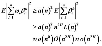
Proof of Theorem 1.1: Given the model where  are covariance-stationary, and for some sufficiently large numbers M and N, it can be shown that any well-diversified portfolio with n numbers of assets,
  ,
,
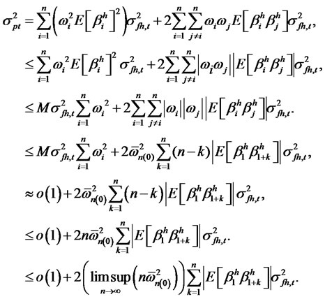
If the hidden factor is non-diversifiable, it is conceivable to have  even when
  Since
Since
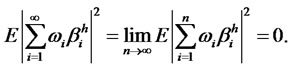
 and if
 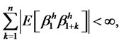 it implies that
 That is, the variance of the well-diversified portfolio will converge to zero. This violates the assumption that the hidden factor is non-diversifiable. Hencethis shows that
 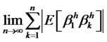 must not be finite if the hidden factor is non-diversifiable. Instead,
In other words, given that  are covariancestationary, the idiosyncratic risk will have a crosssectional long memory. Conversely, if the idiosyncratic hidden factor is of long memory, then it is not W* -diversifiable. Suppose not. Since the definition of diversifiable factor refers to all well-diversified weights in the choice set W*, where
for all well-diversified . Choose one well-diversified portfolio
  with positive weights for all assets, where
  for all
 , and let
  such that
  For any n,
That is to say, the lower bound of the variance of weighted hidden factor loadings does not converge to zero unless it was multiplied by . This violates that

Hence, the hidden factor with assumed long memory should be non-diversifiable.
Proof of Theorem 1.2: Since the test statistic depends only on the sampled covariances (regardless of the underlying process is self-similar with  or it is a fractional-difference model as
 ) and that the hidden factor is stationary, it is easy to set d in the assumptions of L. Giraitis, P. Kokoszaka, R. Leipus, and G. Teyssiere [1] as
  without loss of generality, and for each date t,
 is defined as a consistent estimate for the
  under cross-sectional memory condition in
  as
as . Hence, as
by applying assumption A6 and the continuous mapping. In addition, if there is a non-diversifiable hidden factor in idiosyncratic risk such that the idiosyncratic risk contains long memory as in assumption A5, and ,
,
 it can be shown that
 , where
  is the variance of the partial sums of long memory series and hence,
where  is a fractional Brownian bridge with Hurst coefficient
 . Since the rescaled variance is positive,
  , as
, as ,
,  ,
, .
.
Hence, the test statistic is consistent.
Proof of Theorem 1.3: Denote the fitted asset pricing model (at any time t as we suppress the time index theretofore for simplicity) as
 where
where  is a n-by-1 vector of excess rates of return in n assets,
  is a n-by-p matrix of factor loadings as
  is the element of
  on i-th row and j-th column,
  as the (p + 1) vector of presumed factors,
  is a n-by-1 vector of idiosyncratic risk,
  is a n-by-1 vector of forecast errors conditional on the factors included in model. It suffices to show that the estimate
  is a consistent estimate of
  for each time t. Let
 and
and .
.
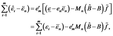
Also let  be a n-by-1 vector with m elements of one’s and
  elements of zero’s, m = 1,2,···,n. Then, let
  be the matrix of consistently estimated factor loadings, it can be shown that
 and the cumulative partial sums as m = 1,2,···,n
where ,
,  is a n-by-n identity matrix. Since
  when estimated consistently,
  and
and  as
as , it is easy to see that
 .
.
Since , let the selection matrices be defined as
 ,
,  , where
  is a
is a  -by-j matrix with zero’s.
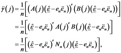
where  is a n-by-n matrix. Hence,
since  and
and ,
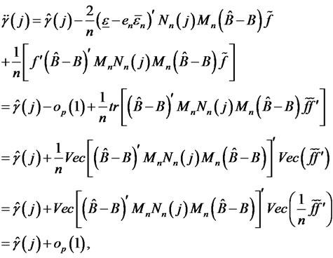
,  is a positive definite finite p-by-p matrix. Hence, given the consistency in estimating cross-sectional auto-covariances using forecast errors, the estimate
  for
for  is also consistent for each time t. Notice that
 under the null hypothesis as
  Hence, in
  the term
  in test statistics will vanish. Using the
  test statistics, this is similar to setting
  as an additional restriction.
Hence, by assumption A6,
for all  this implies that
  In other words, we have
  Therefore,under the null hypothesis,
  test statistic will also converge to the same distribution of
NOTES
1With this definition, we confine the discussion to asset returns with finite second-ordered moment. Further extension is feasible if the infinite variance is introduced in the framework. This, however, requires additional assumptions for the underlying statistical distributions of the stable processes. We leave this for future studies.
2The perceived factors are the proxies for the identified factors of the multifactor pricing model.
4The weights can be shown as  which vary with different sequences of factor loadings
  even for the same hidden factor
 . To be concise, we denote it as
  here. In addition, to avoid the case where the portfolio only consists of a finite number of assets with non-zero weights, we assume that the choices of weights must expand to infinite numbers of assets in the return space where
  -space stands for the metric space with
  -norm
-norm  if
if .
.
5The notation  implies that the limit
  exists for the convergent infinite series of weights.
7To control the decaying rate of the diversifying weights, we need to impose the tail restriction that the weights do not collapse to zero drastically. Otherwise, we would have a degenerated portfolio that consists of infinitely many assets with negligible weights when the number of assets grows. Hence, we include  on the diversifying weights. If
  for all i’s, the decaying rate of
  cannot be greater than
 . The purpose of confining the range of
  to
to  is to control the exponential decaying rate of
 . Otherwise, the bigger
  is, the faster
  will be allowed to decay even when
  is satisfied, making diversification impossible.