Journal of Mathematical Finance
Vol.2 No.2(2012), Article ID:19218,4 pages DOI:10.4236/jmf.2012.22021
A Computational Approach to Financial Option Pricing Using Quasi Monte Carlo Methods via Variance Reduction Techniques
1Department of Applied Mathematics, Faculty of Mathematical Sciences, University of Guilan, Rasht, Iran
2Department of Statistics, Islamic Azad University North Tehran Branch, Tehran, Iran
Email: fmehrdoust@guilan.c.ir, K_fathi@iau-tnb.ac.ir
Received December 10, 2011; revised January 12, 2012; accepted January 12, 2012
Keywords: Financial mathematics; option pricing; Quasi Monte Carlo; variance reduction; Brownian motion; Sobol sequence
ABSTRACT
In this paper, we consider two types of pricing option in financial markets using quasi Monte Carlo algorithm with variance reduction procedures. We evaluate Asian-style and European-style options pricing based on Black-Scholes model. Finally, some numerical results presented.
1. Introduction
The theory of finance, like many areas where advanced mathematics plays an important part, is undergoing a revolution aided and abetted by the computer and proliferation of powerful simulation and symbolic mathematical tools. A fundamental implication of asset pricing theory is that under circumstances, the price of a derivative security can be useful represented as an expected value. Valuing derivatives thus reduces to computing expectations. Therefore, if we were to write the relevant expectation as an integral, we would find that its dimension is large or even infinite. This is precisely the sort of setting in which Monte Carlo and quasi Monte Carlo methods become attractive [1-3]. Monte Carlo and quasi Monte Carlo methods are ubiquitous in applications in the finance and insurance industry. They are often only accessible tol for financial engineers and actuaries when it comes to complicated price or risk computations, in particular for those that are based on many underlying [ref. 2010.Monte quasi]. Since the convergence rate of Monte Carlo methods is generally independent of the number of state variables, it is clear that they become viable as the underlying models (asset prices and volatilities, interest rates) and derivative contracts themselves (defined on path-dependent functions or multiple assets) become more complicated.
The main idea of the Monte Carlo method is to approximate an expected value  by an arithmetic average of the results of a big number of independent experiments which all have the same distribution as X. The basis of this method is one of the most celebrated results of probability theory, the strong law of large numbers. As expected values play a central role in various areas of applications of probabilistic modeling, the Monte Carlo method has a widespread use. Examples of such areas of application are the analysis and design of queuing systems (such as in supermarkets or in large factories), the design of evacuation schemes for buildings, the analysis of the reliability of technical systems, the design of telecommunication networks, the estimation of risks of investments or of insurance portfolios, just to name a few [1,2]. The problem of using Monte Carlo and quasi Monte Carlo methods for computational finance has been extensively studied [4-8].
2. Definition of Financial Mathematics
Let  denote the price of the stock at time t.
Consider a call option granting the holder the right to buy the stock at a fixed price k at a fixed time T in the future; the current time is . If at time T the stock price
  exceeds the stricke price k, the holder exercises the option for a profit of
 ; if on the other hand,
  , the option expires worthless. This is European option, meaning that it can be exercised only at the fixed date T. The payoff to option holder at time is [2]
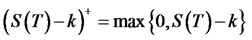 (1)
(1)
The payoff in Asian-style option defined the average level of the underlying asset. This includes, for example, the payoff  with
with
 (2)
(2)
For some fixed set of dates  with the date at which the payoff is received.
One of important model for the dynamics of stock price is Block-Scholes model. This model describes the evaluation of the stock price through the stochastic differential equation
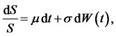 (3)
(3)
where  is a standard Brownian motion. The parameter
  and
and  are continuously compounded interest rate (fixed trend) and volatility of te stock price, respectively.
Now, using Ito’s lemma the equation of the stochastic differential equation as [1]
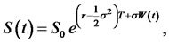 (4)
(4)
with  is the current price of the stock, we may assume it is known. If
  is a standard normal random variable, then the distribution of
  is
is . Therefore, the terminal stoch price as
 (5)
(5)
Based on Block-Scholes model and the risk-neutral model, the total price of (1) becomes
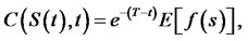 (6)
(6)
where 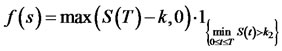 and
and  is 1 if
  holds and zero otherwise. Also,
  are prearranged constants [2].
For a European option pricing we have
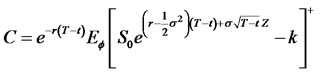 (7)
(7)
where  is the standard normal density.
In Asian-style case, we can write
 (8)
(8)
3. Quasi Monte Carlo Methods and Variance Reduction Techniques
Quasi Monte Carlo methods can be succinctly described as deterministic versions of Monte Carlo methods. Determinism enters in two ways, namely, by working with deterministic points rather than random samples and by the availability of deterministic error bounds instead of the probabilistic Monte Carlo error bounds. The connections between quasi Monte Carlo methods and uniform pseudorandom numbers arise in the theoretical analysis of various methods for the generation of uniform pseudorandom numbers. The pseudorandom sequences simulate random samples from a  distribution and quasi random sequences correspond to samples from a
  distribution. In [5,6] one can find several quasirandom sequences, such as Halton sequences, Sobol sequences, Faure sequences, and Niederreiter sequences.
The Sobol Sequence
The Sobol sequence is defined in base 2. To generate the  component of the points in a Sobol sequence, we need to choose a primitive polynomial of some degree
  in the field
 (9)
(9)
where .
.
The  component of the
  point in a Sobol sequence, is given by
 , (10)
where  are defined as
  and the sequence of positive integer
  defined by the recurrence relation
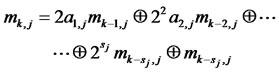 (11)
(11)
where  is the bit by bit exclusive, or operator and
  is the
  digit from the right when
  is written binary [9].
4. Variance Reduction Techniques
Variance reduction techniques are widely used for improving the efficiency of Monte Carlo methods. In this paper, we employ the possibility of using the deterministic versions of some variance reduction techniques (that is, Antithetic variates and Control variates) for the variation reduction in the context of quasi Monte Carlo methods [9]. In the following we will introduce some variance reduction methods.
4.1. Antithetic Variates
The method of antithetic variables is the easiest variance reduction method. It is based on the idea to combine a random choice of points with a systematic one. Its main principle is variance reduction by introducing symmetry [9]. Assume we ant to compute  with
with  a random variable uniformly distributed on
  While the standard (Crude) Monte Carlo estimate would be
 (12)
(12)
with  being independent copies of
 , in the method of antithetic variates we would also use the numbers
  and introduce the antithetic Monte Carlo estimator
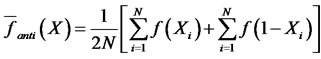 (13)
(13)
Note that  and
and  have the same distributions, both same on the right hand side of equation (12) are unbiased estimators for
 . The variance of antithetic estimator is given by
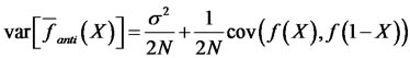
Theorem 1. Let  be a non-decreasing or a non-increasing function and
  be uniformly distributed on
  with
with  being finite. Then we have [9]
In particular, the antithetic Monte Carlo estimator based on  random numbers has a smaller variance than the standard Monte Carlo estimator based on
  random numbers.
4.2. Control Variates
Suppose that we want to estimate  where
where  the output is it of a simulation experiment. Suppose that
  is also an output of the simulation or that we can easily output it if we wish. Then we can construct many unbiased estimators of
  such that
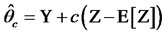 , (14)
where  is some real number. It is clear that
 . We should choose the value of
  such that to minimize
 . Using some calculation implies that the optimal value of
 . For this purpose let
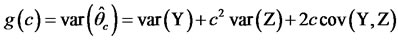
We have
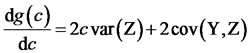 (15)
(15)
By setting (9) to zero, we see that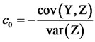 , is critical point of g.
Since , then
  is a local minimum of
 . On the other hand,
  is just a single extreme of g in its domain. Then
  is absolute minimum of g. Thus, with selecting
  the variance
  minimizes, that is
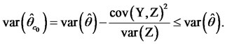 (16)
(16)
We note that for achieving a variance reduction it is only necessary that . (We note that in practice
  never is known and we thus to simulate it). In this case, the random variable
  is called a control variate for random variable Y [10].
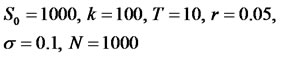
5. Numerical Experiments
In this section, we chose the following values for BlockScholes model for two options pricing, i.e., Europeanstyle and Asian-style. The results in Tables 1 and 2 were obtained using the method as described in equations (7) and (8).
6. Conclusion
This paper presents the computational results for two types of financial option pricing for Block-Scholes model. Based on the results obtained in Tables 1 and 2, the control variates Monte Carlo method is efficient for European and Asian options pricing.
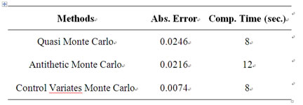
Table 1. Option value error in European-style.
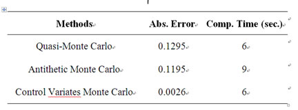
Table 2. Option value error in Asian-style.
7. Acknowledgements
We would like to thank the reviewer for helpful comments and suggestions.
REFERENCES
- P. Glasserman, “Monte Carlo Methods in Financial Mathematics,” Springer-Verlag, New York, 2004.
- J. S. Dagpunar, “Simulation and Monte Carlo with Applications in Finance and MCMC,” John Wiley & Sons, New York, 2007.
- V. N. Alexandrov, C. G. Martel and J. Strabburg, “Monte Carlo Scalable Algorithms for Computational Finance,” Procedia Computer Science, Vol. 4, 2011, pp. 1798-1715. doi:10.1016/j.procs.2011.04.185
- L. Cao and Z. F. Gue, “A Comparison of Gradient Estimation Techniques for European Call Options,” Accounting & Taxation, Fothcoming, 2011.
- L. Cao and Z. F. Gue, “A Comparison of Delta Hedging under Two Price Distribution Assumptions by Likelihood Ratio,” International Journal of Business and Finance Research, Forthcoming, 2011.
- L. Cao and Z. F. Gue, “Delata Hedging with Deltas from a Geometric Brownian Motion Process,” Proceeding Conference on Applied Financial Economic, Samos Island, March 2011.
- L. Cao and Z. F. Gue, “Applying Gradient Estimation Technique to Estimate Gradients of European Call Following Variance-Gamma,” Global Conference on Business and Finance Proceeding, Vol. 6, No. 2, 2011, pp. 12-18.
- M. Davis, “Mathematics of Financial Markets,” Supported by FWF, 2009.
- C. Lemieux, “Monte Carlo and Quasi Monte Carlo Sampling,” Springer Science, New York, 2009.
- B. Fathi Vajargah and F. Mehrdoust, A. Pourdarvish and F. Norouz, “Some New Advantages on Monte Carlo Integration Using Variance Reduction Procedures,” International Journal of Advanced Research in Computer Science, Vol. 1, No. 4, 2011.