Open Journal of Statistics
Vol.3 No.2(2013), Article ID:30327,11 pages DOI:10.4236/ojs.2013.32013
Bayesian Estimation for GEV-B-Spline Model
1Center Eau Terre Environnement, Institut national de la Recherche Scientifique Québec, Canada
2Département de Mathématique et de Statistique, Université de Moncton, Moncton, Canada
3Masdar Institue of Science and Technology, Abu Dhabi, UAE
Email: Bouchra.nasri@ete.inrs.ca, salah-eddine.el.adlouni@umoncton.ca, touarda@masdar.ac.ae
Copyright © 2013 Bouchra Nasri et al. This is an open access article distributed under the Creative Commons Attribution License, which permits unrestricted use, distribution, and reproduction in any medium, provided the original work is properly cited.
Received December 10, 2012; revised January 11, 2013; accepted January 25, 2013
Keywords: GEV; Bayesien; B-Spline; Nonlinearity; Covariate; Non-Stationarity
ABSTRACT
The stationarity hypothesis is essential in hydrological frequency analysis and statistical inference. This assumption is often not fulfilled for large observed datasets, especially in the case of hydro-climatic variables. The Generalized Extreme Value distribution with covariates allows to model data in the presence of non-stationarity and/or dependence on covariates. Linear and non-linear dependence structures have been proposed with the corresponding fitting approach. The objective of the present study is to develop the GEV model with B-Spline in a Bayesian framework. A Markov Chain Monte Carlo (MCMC) algorithm has been developed to estimate quantiles and their posterior distributions. The methods are tested and illustrated using simulated data and applied to meteorological data. Results indicate the better performance of the proposed Bayesian method for rainfall quantile estimation according to BIAS and RMSE criteria especially for high return period events.
1. Introduction
Many fields of modern science and engineering have to deal with rare events with significant consequences. Extreme value theory (EVT) allows to providing the basis for the statistical modeling of such extremes. The main result of EVT shows that the maxima, of Independent and Identically Distributed (i.i.d.) events, are asymptotically Generalized Extreme Value (GEV) distributed [1]. In practice, the hypotheses of the EVT are, generally, not fulfilled, and a classical frequency analysis, of independent, homogeneous and stationary samples, is considered with a large range of probability distributions to estimate the occurrence of extreme events. A number of methods have been proposed to estimate GEV distribution’s parameters; such as the method of moments (MM) [2,3], maximum likelihood (ML) [4] and the method of probability weighted moments [5].
The Stationarity assumption is essential to carry out a statistical frequency analysis. However, in many fields, such as hydroclimatology, observed data series are not stationary [6,7]. For hydrological datasets, two main types of non-stationarity have been observed due to temporal trends or cycles corresponding to the effect of other covariates. The second kind of non-stationarity, has been largely studied during the last decade through the GEV model with covariates [8-14] for local frequency analysis and [15,16] for regional analysis.
Taking into account the effect of a covariate can be considered in a polynomial form [9,11,17]. These polynomial forms for estimating the GEV parameters were developed by the introduction of covariates in a polynomial form such as a linear or quadratic function. However, the dependence between covariates and variables of interest can take different structures.
[18] suggested the use of semi-parametric functions such as smoothing splines to estimate the relationship between the parameters and covariates. The smoothing splines are based on the minimization of the penalized sum of the squared errors and the choice of the smoothing parameter [19]. The main disadvantages of this type of function are that inference, often through the confidence bands, is not straightforward and that a smoothing which parameter needs to be specified at the beginning [20]. A smoothing-based B-spline function resolves these problems and presents several others advantages.
B-spline functions are linear combinations of non negative piecewise-polynomial real functions. A B-spline function does not depend on the response variable, or the variable of interested, but depend only on: 1) the support of the covariates, 2) the number and position of knots and 3) the degree of B-Spline function [19]. The above advantages of B-Spline functions make it an appropriate option to be used in the GEV model with covariates to estimate the quantiles conditionally to given factors. The GEV model with B-spline called mixed GEV-B-Spline model, is rigorous and flexible and allows to fit a large number of dependence structures [18,21]. [18] describes smooth non-stationary generalized additive modeling for sample extremes, in which spline smoothers are incorporated into models for exceedances over high thresholds with the Generalized Pareto distribution. They developed the maximum penalized likelihood estimation approach with uncertainty assessed by using differences of deviances and bootstrap simulation.
The main objective of the present study is to develop the Generalized Extreme Value model with covariates where the dependence structure is represented by B-spline functions in a Bayesian framework. Prior distributions have been proposed and the posterior distribution is simulated through the Metropolis Hasting (MH) algorithm based on the Monte Carlo Markov Chain (MCMC) method.
In the next section, the theoretical development of the Bayesian method of parameter estimation is discussed. A case study is then presented in Section 3. A comparison between of the proposed Bayesian approach with classical estimation methods such as the method of moments and the maximum likelihood method is presented in the third section. The last section corresponds to the conclusions and recommendations for future work.
2. Bayesian GEV-B-Spline Model
2.1. GEV Distribution
The extreme value theory introduced by [22] shows that the limiting distribution of the maximum is one of the following distributions: Gumbel, Frechet or Weibull. These three distributions can be grouped in a single Generalized Extreme Value (GEV) distribution:
 (1)
(1)
• The Gumbel distribution has two parameters defined on R, the distribution function is obtained by tendering .
.
• The Fréchet distribution has three parameters defined on the interval , obtained for
 .
.
• The Weibull distribution has three parameters defined on the interval , obtained for
 .
.
Considering ![]() a random variable following the GEV distribution and
a random variable following the GEV distribution and  the time before the event
 . Then
  is distributed according to a Geometric distribution with a parameter
 .
.
Let  be i.i.d. random variables from the GEV distribution. The probability that
  is given by:
 (2)
(2)
with:
 (3)
(3)
Since the variable Y follows the GEV distribution with F as a repartition function. Equation (3) becomes:
 (4)
(4)
So the quantile  of the GEV distribution is:
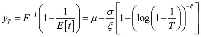 (5)
(5)
In the non-stationary case, the parameters of the GEV are functions of time or other covariates. Consequently the quantile  depends on these covariates. In the present study, the parameters
 ![]() and
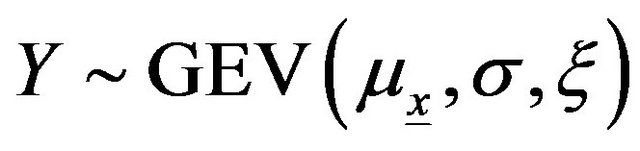
and  are supposed constant. Let Y be a random variable that follows the
 , and
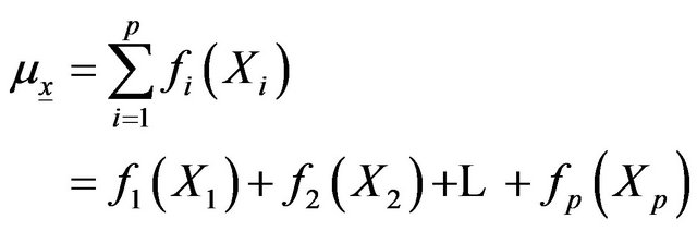
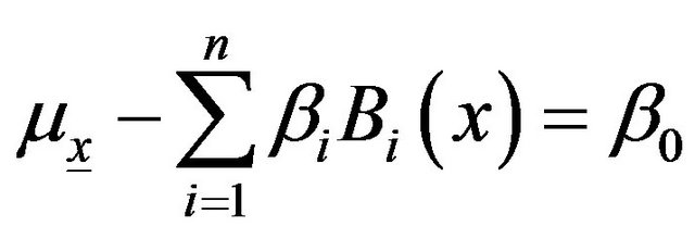
, and  a vector of covariates. The location parameter of the GEV model is a function of covariates:
 (6)
(6)
where  represents the function that describes the relationship between the parameter and the covariate Xi.
In the classical GEV model with covariates, dependence is represented through polynomial functions of linear or quadratic forms. In the following paragraph, we present the GEV model with covariates where the dependence structure is given by B-Splines. This model will be called GEV-B-Spline.
2.2. The GEV-B-Spline Model
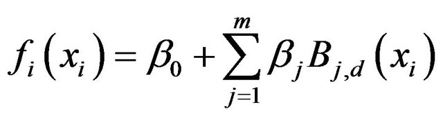
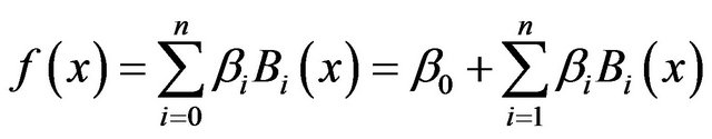
The function  can be decomposed in the form of basic spline functions:
 (7)
(7)
where
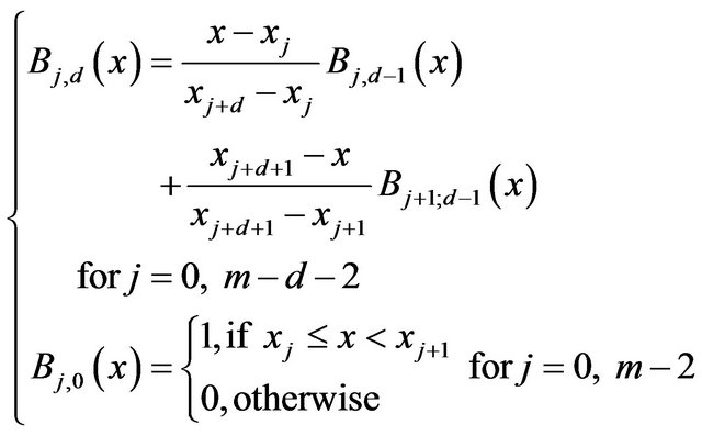 (8)
(8)
 is a polynomial of degree d on each interval and m is the number of control points.
Hence, the Equation (6) becomes
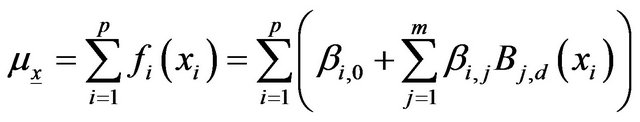 (9)
(9)
The matrix form of Equations (8) and (9) gives
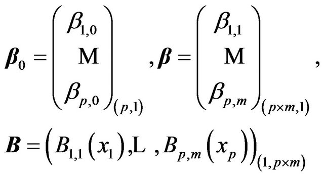 (10)
(10)
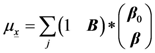 (11)
(11)
where 1 is the unit vector of size p.
2.3. The GEV-B-Spline Model in Bayesian Framework
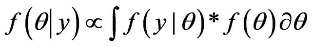
The GEV-B-Spline is considered in a fully Bayesian framework. For a given parameter prior distribution,  , the Bayes theorem allows to define the posterior distribution:
 (12)
(12)
where
is the vector of the parameters, and  and
and ![]() are the hyper-parameters of the location parameter.
are the hyper-parameters of the location parameter.
[23] proposed the Beta  distribution as a prior distribution for the shape parameter of a stationary GEV model, in order to avoid irrational estimations of the shape parameter. In the present study, we considered an equivalent prior for the shape parameter; it is the normal distribution with mean 0.1 and variance 0.12.
[11] adopted this prior distribution for the GEV model with covariates with polynomial dependence. Other studies have suggested adopting the normal distribution to model the hyper parameters of the location parameter for the GEV model with covariates and B-Spline dependence [21,24].
 (13)
(13)
For the scale parameter, we used a non informative prior distribution 1/σ
The posterior distribution of  is written as follows:
 (14)
(14)
then
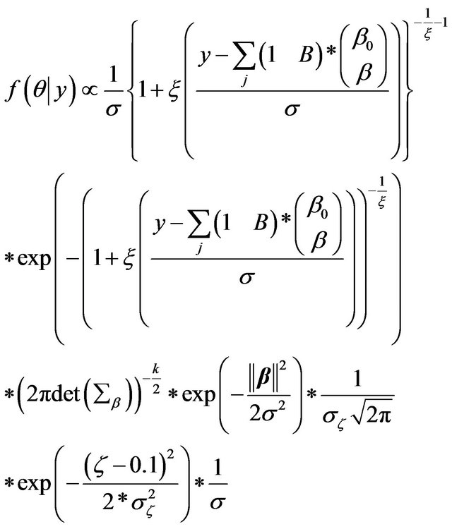 (15)
(15)
The posterior distribution  is a function of the hyperparameters
Considering a simple case of one covariate and m = 1 and d = 1, Equation (15) becomes:
 (16)
(16)
where
 (17)
(17)
![]() and
and ![]() are the parameter set by the prior distribution. To estimate the above function, initial values of the parameters
are the parameter set by the prior distribution. To estimate the above function, initial values of the parameters  then should be given in order to simulate their joint posterior distribution by a MCMC algorithm. The marginal distributions of the parameters can be deduced by integrating Equation (15), with respect to the rest of the parameter vector:
 (18)
(18)
The following section presents the details of the proposed MCMC algorithm to estimate the GEV-B-Spline parameter and quantile distributions.
2.4. MCMC Algorithm for the GEV-B-Spline Model
The MCMC method constitutes an alternative to the numerical methods, especially in Bayesian statistical analysis. The basic idea of the MCMC method is, for each parameter, to construct a Markov chain with the posterior distribution being a stationary and ergodic distribution. After running the Markov chain, of size , for a given burn-in period
 , one obtains a sample from the posterior distribution
 . One popular method for constructing a Markov chain is via the Metropolis-Hastings (MH) algorithm [25,26]. For the GML method, we simulated realizations from the posterior distribution by way of a single-component MH algorithm [27]. Each parameter was updated using a random-walk Metropolis algorithm with a Gaussian proposal density centered at the current state of the chain. Some methods to assess the convergence of the MCMC methods make it possible to determine the length of the chain and the burn-in time such as Raftery & Lewis and Subsampling methods [28]. In all cases, the convergence methods indicated that the Markov chains converged within a few iterations. In this study, we considered chains of size
  and a burn-in period of
  runs. In every case, a sample of
  values is collected from the posterior of each of the elements of
 . The GML corresponds to the mode of the empirical posterior distribution obtained from the
  values generated by the MCMC algorithm.
The MCMC algorithm produces also the conditional quantile distribution for an observed value , of the covariate
![]() . Indeed, for each iteration
. Indeed, for each iteration  of the MCMC algorithm
 , the quantiles with non-exceedance probability
 ,
,  corresponding to the parameter vector
 , are computed using the inverse of the cumulative distribution function of the GEV distribution:
 (19)
(19)
where  is the position parameter conditional on the particular value
  of
of . Several statistical characteristics of the conditional quantile distribution can be determined from the values
 , such as the mean, the mode or the confidence interval. Principal step of the MH algorithm can be summarized as follows [13]:
1) Choose a proposal distribution q;
2) Given the current state![]() , generate
, generate  from
from ;
;
3) Accept  with probability

3. Case Study
3.1. Dataset
The proposed model is considered to model the maximum annual rainfall (MAR) at Randsburg station (047253), California for the period of 1938-2007. The Randsburg station is located in the south east of the state of California . Figure 1 illustrates the geographic location of the Randsburg station. Figure 2
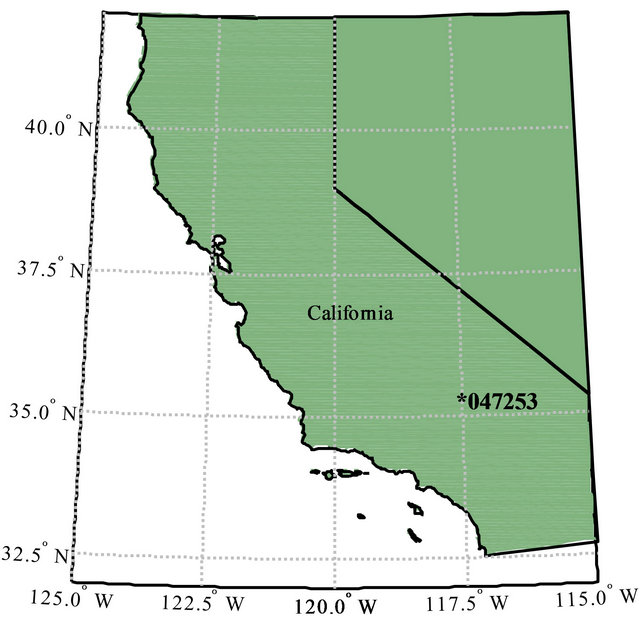
Figure 1. Geographic location of the Randsburg station.

Figure 2. Variation of maximum annual rainfall.
shows the 70-year variation of MAR at Randsburg Station.
We consider the 70-year Southern Oscillation Index (SOI) and Pacific Decadal Oscillation (PDO) time series as covariates for MAR non-stationary quantile estimation. The SOI and PDO describe the pressure and temperature anomalies over the Pacific Ocean and have a clear impact on water systems in North America [14,29]. By using SOI and PDO as covariates in estimating the parameters of the GEV-B-Spline model, we will take into account the effect of multiannual climate fluctuations on extreme rainfall events. We first apply the Mann Kendall test to examine the existence of non-stationarity (Trend) in MAR time series. The result shows that the MAR is not stationary at 1% significant level. The Spearman’s rho correlation coefficient between the covariates and MAR is −0.52 and 0.51 for SOI and PDO respectively. These values are significant at the 5% level. Figure 3 shows the variation of maximum annual rainfall against SOI and PDO.
3.2. Model Development
For model development, the following function is first fitted:
GEV-B-Spline

 are independent spline functions, for which the degree and the number of nodes should be determined. In this application the number of nodes and the degree of the function are both chosen to take the value 3.
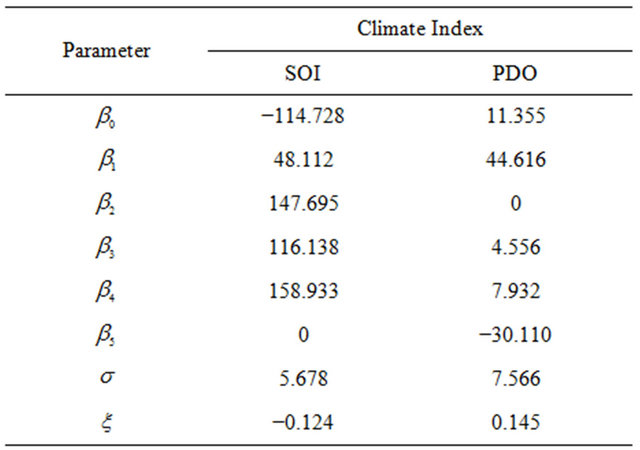
Table 1 shows the GEV-Spline parameters fitted to SOI and PDO time series using a Bayesian method. Figures 4 and 5 show the estimated 2, 20 and 50-year return period maximum rainfall quantiles as function of the covariates (SOI and PDO). It can be seen that, generally, the SOI has a negative correlation with precipitation, while PDO is positively correlated with precipitation. The negative values of SOI (e.g. El Nino phase) and positive values of PDO (Warm Phase of PDO) coincide with the relatively high MAR observations. MAR quantiles increase slowly with increasing PDO values and then increase exponentially for PDO values greater than 1. On the other hand, different inflexion points, in the relationship between SOI and MAR are observed (for example at SOI = −1.5, SOI = 0 and SOI = 1.5), indicating a more complex relationship between SOI and MAR than between PDO and MAR.
4. Parameter Estimation Comparison
In this section, we propose a comparison of the Bayesian parameter estimation method for the GEV-B-Spline model (BAYES) and other estimation methods such as the conventional method of moments (MM) and the method of maximum likelihood (ML). The theoretical backgrounds of these two methods for the GEV-B-Spline model are presented in Appendices 1 and 2, respectively. The comparison of these methods is carried out based on a simulation of MAR-SOI relationship only. The quantile with a non-exceedance probability 1 − p is computed for the maximum SOI using the parameters given by the Bayesian method (Table 1). The objective is to compare the quantile estimation methods for the quantiles estimated from 1000 samples of size  generated from each estimation method. The parameter values chosen for simulation are
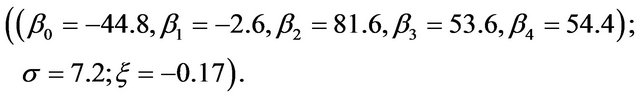

Figure 3. Annual maximum rainfall against SOI and PDO index.
Table 1. Bayesian estimation of the parameters of the model.
The comparison is carried out using the bias and the root mean square error (RMSE) of quantile estimations at non-exceedance probabilities, 1 − p = 0.5, 0.8, 0.9, 0.99 corresponding to return periods of 2, 5, 10, 100. The results are given in Table 2.
Results show that the Bayesian estimation for the GEV-B-Spline model in all cases represents the best results. However, this estimation method requires large time-consuming numerical calculations and does not meet a convergence point easily. For our case, the MCMC method details, such as the choice of numerical method burning period and number of iterations are the key points to the convergence of the MCMC algorithm. On the other hand, even if the method of moments is the easiest method to implement, the corresponding results are largely unsatisfactory. The method of maximum likelihood, however, is a compromise between the other two methods. It is interesting to note that for the case of low return periods, i.e.  and
and  years, the maximum likelihood method gives almost comparable results with the Bayesian estimation. However, the error of the ML method increases rapidly with the increase in the return period and the method becomes increasingly less effective. Therefore, the Bayesian method leads to a superior performance for the estimation of the extreme rainfall quantiles for all return periods. The Bayesian method offers also a general framework to combine observed and subjective information and the possibility to estimate the entire predictive distribution of the parameters and quantiles.
5. Conclusions and Recommendations
Statistical risk assessment is of great importance in hydrology and many other fields of applied statistics. The last two decades have witnessed the development of a number of statistical modeling approaches for extreme values in the presence of non-stationarity or dependence on covariates. The GEV-B-Spline model which takes into account the non-stationarity and nonlinearity offers a great flexibility and takes into account the heavy tailed character of the extreme distribution. The present study proposes a Bayesian estimation framework of the GEV-

Figure 4. GEV-B-Spline estimators of the 2, 20 and 50-year return period quantiles conditional upon SOI.
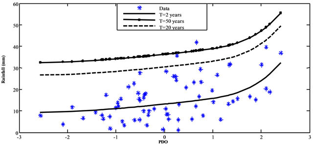
Figure 5. GEV-B-Spline estimators of the 2, 20 and 50-year return period quantiles conditional upon PDO.
Table 2. Comparison of estimation methods.

B-spline model for hydro-meteorological variables. The Bayesian approach is general, flexible and connected with the decision theory. It combines observed and prior information, estimates the entire posterior distribution of the parameters and quantiles and thus allows to estimate the credibility intervals.
Results of the simulated data show the advantage of the proposed method for quantile estimation of an extreme variable such as maximum rainfall especially for high return period.
The evaluation for the quantile uncertainty using BIAS and RMSE criteria also indicated the superiority of the proposed method in comparison to other estimation methods, especially for high return period quantile estimation. However, the uncertainty of quantile estimation of low return periods does not show a significant difference between the bayesian and the maximum likelihood method. On the other hand, one can see that the numerical calculation is the main disadvantage of these types of models when the number of covariates increases which may lead to divergence problem. The quantile regression model can be a good alternative to overcome this problem [30,31]. Therefore, future work can focus on the comparison of extreme value models with regression quantiles in order to use different covariates in quantile estimations.
REFERENCES
- A. F. Jenkinson, “The Frequency Distribution of the Annual Maximum (or Minimum) of Meteorological Elements,” Quarterly Journal of the Royal Meteorological Society, Vol. 81, No. 348, 1955, pp. 158-171. doi:10.1002/qj.49708134804
- T. N. Thiele, “Theory of Observations,” C. and E. Layton, London, 1903, pp. 165-308.
- R. A. Fisher, “Moments and Product Moments of Sampling Distributions,” Proceedings of the London Mathematical Society, Vol. 30, No. 1, 1929, pp. 199-238. doi:10.1112/plms/s2-30.1.199
- R. L. Smith, “Maximum Likelihood Estimation in a Class of Non-Regular Cases,” Biometrika, Vol. 72, No. 1, 1985, pp. 67-90. doi:10.1093/biomet/72.1.67
- J. Hosking, “L-Moments: Analysis and Estimation of Distributions Using Linear Combinations of Order Statistics,” Journal of the Royal Statistical Society, Series B, Vol. 52, No. 1, 1990, pp. 105-124.
- D. J. Dupuis, “Modeling Waves of Extreme Temperature: The Changing Tails of Four Cities,” Journal of the American Statistical Association, Vol. 107, No. 497, 2012, pp. 24-39. doi:10.1080/01621459.2011.643732
- P. C. D. Milly, J. Betancourt, M. Falkenmark, R. M. Hirsch, Z. W. Kundzewicz, D. P. Lettenmaier and R. J. Stouffer, “Stationarity Is Dead: Whither Water Management?” Science, Vol. 319, No. 5863, 2008, pp. 573-574. doi:10.1126/science.1151915
- J. R. Olsen, J. R. Stedinger, N. C. Matalas and E. Z. Stakhiv, “Climate Variability and Flood Frequency Estimation for the Upper Mississippi and Lower Missouri Rivers,” Journal of the American Water Resources Association, Vol. 35, No. 6, 1999, pp. 1509-1524. doi:10.1111/j.1752-1688.1999.tb04234.x
- S. Coles, “An Introduction to Statistical Modeling of Extreme Values,” Springer, London, 2001.
- J. M. Cunderlik, V. Jourdain, T. B. M. J. Ouarda and B. Bobée, “Local Non-Stationary Flood-Duration-Frequency Modeling,” Canadian Water Resources Journal, Vol. 32, No. 1, 2007, pp. 43-58. doi:10.4296/cwrj3201043
- S. El Adlouni, T. B. M. J. Ouarda, X. Zhang, R. Roy and B. Bobee, “Generalized Maximum Likelihood Estimators for the Nonstationary Generalized Extreme Value Model,” Water Resources Research, Vol. 43, No. 3, 2007, W03410. doi:10.1029/2005WR004545
- Y. Hundecha, T. B. M. J. Ouarda and A. Bárdossy, “Regional Estimation of Parameters of a Rainfall-Runoff Model at Ungauged Watersheds Using the Spatial Structures of the Parameters within a Canonical PhysiographicClimatic Space,” Water Resources Research, Vol. 44, No. 1, 2008, W01427. doi:10.1029/2006WR005439
- S. El Adlouni and T. B. M. J. Ouarda, “Joint Bayesian Model Selection and Parameter Estimation of the Generalized Extreme Value Model with Covariates Using Birth-Death Markov Chain Monte Carlo,” Water Resources Research, Vol. 45, No. 6, 2009, W06403. doi:10.1029/2007WR006427
- A. Cannon, “A Flexible Nonlinear Modelling Framework for Nonstationary Generalized Extreme Value Analysis in Hydroclimatology,” Hydrological Process, Vol. 24, No. 6, 2010, pp. 673-685. doi:10.1002/hyp.7506
- J. M. Cunderlik and T. B. M. J. Ouarda, “Regional FloodDuration—Frequency Modeling in a Changing Environment,” Journal of Hydrology, Vol. 318, No. 1-4, 2006, pp. 276-291. doi:10.1016/j.jhydrol.2005.06.020
- M. Leclerc and T. B. M. J. Ouarda, “Non-Stationary Regional Flood Frequency Analysis at Ungauged Sites,” Journal of Hydrology, Vol. 343, No. 3-4, 2007, pp. 254- 265. doi:10.1016/j.jhydrol.2007.06.021
- S. El Adlouni and T. B. M. J. Ouarda, “Comparison of Methods for Estimating the Parameters of the Non-Stationary GEV Model,” Revue des Sciences de l’Eau, Vol. 21, No. 1, 2008, pp. 35-50.
- V. Chavez-Demoulin and A. Davison, “Generalized Additive Modeling of Sample Extremes,” Applied Statistics, Vol. 54, No. 1, 2005, pp. 207-222. doi:10.1111/j.1467-9876.2005.00479.x
- C. De Boor, “A Practical Guide to Spline,” Springer, London, 2001, 208 pp.
- H. G. Müller and J. L. Wang, “Density and Failure Rate Estimation,” In: F. Ruggeri, R. Kenett and F. W. Faltin, Eds., Encyclopedia of Statistics in Quality and Reliability, Wiley, Chichester, 2007, pp. 517-522.
- S. A. Padoan and M. P. Wand, “Mixed Model-Based Additive Models for Sample Extremes Statistics and Probability,” Letters, Vol. 78, No. 17, 2008, pp. 2850-2858.
- R. A. Fisher and L. H. C. Tippett, “Limiting Forms of the Frequency Distribution of the Largest or Smallest Member of a Sample,” Proceedings of the Cambridge Philosophical Society, Vol. 24, No. 2, 1928, pp. 180-190. doi:10.1017/S0305004100015681
- E. S. Martins and J. R. Stedinger, “Generalized Maximum Likelihood GEV Quantile Estimators for Hydrologic Data,” Water Resources Research, Vol. 36, No. 3, 2000, pp. 737-744. doi:10.1029/1999WR900330
- S. Neville, M. J. Palmer and M. P. Wand, “Generalised Extreme Value Geoadditive Model Analysis via Mean Field Variational Bayes,” Australian and New Zealand Journal of Statistics, Vol. 53, No. 3, 2011, pp. 305-330. doi:10.1111/j.1467-842X.2011.00637.x
- N. Metropolis, A. Rosenbluth, M. Rosenbluth, A. Teller and E. Teller, “Equation of State Calculations by Fast Computing Machines,” The Journal of Chemical Physics, Vol. 21, No. 6, 1953, pp. 1087-1092.
- W. K. Hastings, “Monte Carlo Sampling Methods Using Markov Chains and Their Applications,” Biometrika, Vol. 57, No. 1, 1970, pp. 97-109. doi:10.1093/biomet/57.1.97
- W. R. Gilks, S. Richardson and D. J. Spiegelhalter, “Markov Chain Monte Carlo in Practice,” Chapman and Hall, London, 1996.
- S. El Adlouni, A. C. Favre and B. Bobée, “Comparison of Methodologies to Assess the Convergence of Markov Chain Monte Carlo Methods,” Computational Statistics and Data Analysis, Vol. 50, No. 10, 2006, pp. 2685-2701. doi:10.1016/j.csda.2005.04.018
- D. P. Brown and A. C. Comrie, “Sub-Regional Seasonal Precipitation Linkages to SOI and PDO in the Southwest United States,” Atmospheric Science Letters, Vol. 3, No. 2-4, 2002, pp. 94-102. doi:10.1006/asle.2002.0057
- M. Buchinsky, “The Dynamics of Changes in the Female Wage Distribution in the USA: A Quantile Regression Approach,” Journal of Applied Econometrics, Vol. 13, No. 1, 1998, pp. 1-30.
- T. H. Jagger and B. E. James, “Climatology Models for Extreme Hurricane Winds near the United States,” Journal of Climate, Vol. 19, No. 13, 2006, pp. 3220-3236. doi:10.1175/JCLI3913.1
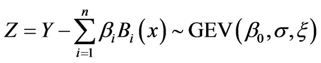
Appendix 1: GEV-B-Spline Moment
Let Y be a random variable that follows a GEV distribution therefore:
 (A1)
(A1)
With  is a parameter that depends on a covariate X.
 (A2)
(A2)
B is a spline basis function.
Where
 (A3)
(A3)
And thus
 (A4)
(A4)
Then
 (A5)
(A5)
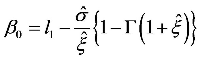
The following equations are used to estimate the parameters :
:
 (A6)
(A6)
 (A7)
(A7)
 (A8)
(A8)
With
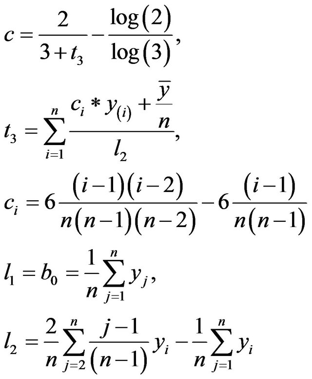 (A9)
(A9)
The other  values are estimated using the linear regression between Y and the basis matrix B of the B-spline corresponding to the covariates.
Appendix 2: GEV-B-Spline Maximum Likelihood
Let Y be a random variable that follows a GEV distribution therefore:
 (A10)
(A10)
With  is a parameter that depends on a covariate X.
 (A11)
(A11)
B is a spline basis function.
The maximum likelihood (ML) function is written as
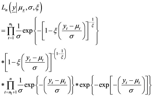
(A12)
 is the number of observations when
 .
.
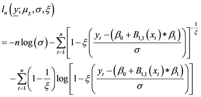
In the case of , the log-likelihood function is:
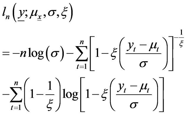 (A13)
(A13)
The ML estimators are the solution of an equation system formed by setting to zero the partial derivates of (A13) with respect to each parameter.
In the case of one covariate and , we have 4 parameters to estimate
(A14)
The ML estimators of the parameter  are the solution of the following system:
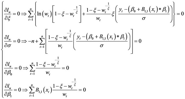 (A15)
(A15)
where
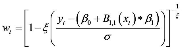 (A16)
(A16)
Numerical methods must be used to solve the system (A15). In the present study we used the Newton Raphson method.
NOTES
*Corresponding author.