¹Business School, The University of Edinburgh, Edinburgh, UK

²Business School, ESC Rennes, Rennes, France

³School of Management and Languages, Heriot-Watt University, Edinburgh, UK

⁴National Graduate Institute for Policy Studies, Tokyo, Japan

Email: ^*Jamal.Ouenniche@ed.ac.uk

Copyright © 2014 by authors and Scientific Research Publishing Inc.

This work is licensed under the Creative Commons Attribution International License (CC BY).

http://creativecommons.org/licenses/by/4.0/

Received 27 May 2014; revised 30 June 2014; accepted 7 July 2014

Abstract

With the increasing number of quantitative models available to forecast the volatility of crude oil prices, the assessment of the relative performance of competing models becomes a critical task. Our survey of the literature revealed that most studies tend to use several performance criteria to evaluate the performance of competing forecasting models; however, models are compared to each other using a single criterion at a time, which often leads to different rankings for different criteria—A situation where one cannot make an informed decision as to which model performs best when taking all criteria into account. In order to overcome this methodological problem, Xu and Ouenniche [1] proposed a multidimensional framework based on an input-oriented radial super-efficiency Data Envelopment Analysis (DEA) model to rank order competing forecasting models of crude oil prices’ volatility. However, their approach suffers from a number of issues. In this paper, we overcome such issues by proposing an alternative framework.

Keywords: Forecasting Crude Oil Prices’ Volatility, Performance Evaluation, Slacks-Based Measure (SBM), Data Envelopment Analysis (DEA), Commodity and Energy Markets

1. Introduction

Oil is an important source of energy that drives modern economies. Changes in oil prices may lead to a substantial impact on such economies; therefore, the proactive knowledge of future movements of oil prices can lead to better decisions at various levels of governments, central banks, and the private sector. In an attempt to gain knowledge on future movements of oil prices, the forecasting of both the level and the volatility of oil prices proves useful. In this paper, we focus on the volatility of oil prices, as forecasts of oil prices’ volatility is an important input to many decision making processes, see, for example, Hamilton [2] and Kilian [3] . First, crude oil prices’ changes tend to negatively affect oil importing economies as a result of increased production costs or decreased production output; therefore, reliable forecasts of oil prices’ volatility are crucial for setting up levels of countries’ oil reserves as a tool for mitigating the negative impact on the economy. Second, central banks take explicit account of the volatility of commodities in establishing their monetary policies; therefore, reliable forecasts of oil prices’ volatility are crucial for macroeconomic policy makers in setting policies to stabilize the economy. Third, oil prices’ volatility tends to raise uncertainty, which affects consumers’ consumption and investment behaviour and often results in reduced or postponed purchases of goods and investments in equipment. Fourth, the financial industry standard approach to investment risk management is to model risk within a parametric approach framework by using value-at-risk (VaR) as a proxy to measure the risk of financial instruments (e.g., stocks, bonds, commodities including crude oil, and futures and options), which requires a reliable estimate of volatility. Fifth, forecasting oil prices’ volatility is a critical activity for investors faced with a massive growth in the trading of crude oil and its underlying derivative securities; for instance, investors or portfolio managers need to forecast the expected volatility over the lifetime of the future or option contract to assist them in designing hedging strategies and in adjusting their investment portfolios when the crude oil market becomes very unstable.

Given the importance of crude oil prices’ volatility, it has attracted considerable attention from governments, investors, analysts, and academics. Most studies tend to analyze the behaviour of oil prices’ volatility and its causes or to propose better volatility forecasting models. Although a relatively large number of models are available to forecast the volatility of crude oil prices, their relative performance evaluation has not attracted as much attention as it deserves. To be more specific, our survey of the literature revealed that most studies tend to use several performance criteria and, for each criterion, one or several metrics to evaluate the performance of competing forecasting models; however, the assessment exercise is typically restricted to the ranking of models by measure. As a consequence, conflicting results about the performance of specific forecasting models are often reported in that some models perform better than others with respect to a specific criterion, but worse with respect to other criteria; thus, leading to a situation where one cannot make an informed decision as to which model performs best overall when taking all criteria into account―see, for example, Sadorsky [4] [5] , Agnolucci [6] , and Marzo and Zagaglia [7] . Xu and Ouenniche [1] highlighted this issue faced by the forecasting community; namely, the fact that the current methodology for assessing the relative performance of competing forecasting models is unidimensional in nature (i.e., models are compared to each other using a single measure of a single criterion at a time). In order to overcome this methodological issue, they proposed a super-efficiency DEA framework for assessing the relative performance of competing forecasting models of oil prices’ volatility, which is based on the super efficiency model of Andersen and Peterson [8] ; namely, BCC-based super-efficiency model, where BCC refers to the DEA model proposed by Banker, Charnes and Cooper [9] . Their multi-criteria framework allows one to obtain a single ranking that takes account of several performance criteria; however, it suffers from a number of issues. First, under the variable returns-to-scale (VRS) assumption, input-oriented efficiency scores can be different from output-oriented efficiency scores, which may lead to different rankings. Second, radial super-efficiency DEA models (e.g., BCC-based super-efficiency model) may be infeasible for some efficient decision making units; therefore, ties would persist in the rankings. Third, radial super-efficiency DEA models ignore potential slacks in inputs and outputs and thus may over-estimate the efficiency score, on one hand, and could only take account of technical efficiency (i.e. CCR score, where CCR refers to the basic DEA model proposed by Charnes, Cooper and Rhodes, [10] ), pure technical efficiency (i.e., BCC score), and scale efficiency (i.e., ratio of CCR score to BCC score); therefore, they ignore or fail to provide mix efficiency (i.e., ratio of SBM score to CCR score, where SBM refers to the slacks-based DEA model proposed by Tone [11] ), on the other hand. Finally, in many applications such as ours, the choice of an orientation in DEA is rather superfluous. In this paper, we overcome these issues by proposing an orientation-free super-efficiency DEA framework; namely, a slacks-based super-efficiency DEA framework for assessing the relative performance of competing volatility forecasting models.

The remainder of this paper is organized as follows. In Section 2, we describe the application context of the proposed multidimensional framework for assessing the relative performance of competing forecasting models; that is, crude oil prices’ volatility. In Section 3, we briefly review the basic concepts of DEA and propose an improved DEA framework to evaluate the relative performance of competing forecasting models for crude oil prices volatility. In Section 4, we present and discuss our empirical results. Finally, Section 5 concludes the paper.

2. Crude Oil Volatility

Crude oil is one of the most important sources of energy and its price has undergone large and persistent fluctuations and seems greatly influenced by exogenous events. In general, global macroeconomic conditions and political instabilities in both OPEC regions and non-OPEC regions are believed to have a substantial impact on oil supply and demand and subsequently on its prices (e.g., Hamilton [2] ; Kilian [3] ). Given the volatile nature of the oil market, a reliable forecast of oil price volatility is an important input to many decision making processes such as macroeconomic policy making, risk management, options pricing, and portfolio management.

As far as the literature on forecasting oil prices’ volatility is concerned, quantitative forecasting models could be divided into three main categories; namely, time series volatility models (Sadorsky [4] [5] ; Agnolucci [6] ; Kang et al. [12] , Marzo and Zagaglia [7] ; Wang and Wu [13] ), implied volatility models (Day and Lewis [14] ; Agnolucci [6] ), and hybrid models (Fong and See [15] ; Nomikos and Pouliasis [16] ). Time series volatility models can be further decomposed into three sub-categories; namely, historical volatility models, generalized autoregressive conditional heteroscedasticity (GARCH) models, and stochastic volatility (SV) models. Historical volatility models are averaging methods that use volatility estimates (e.g., standard deviation of past returns over a fixed interval) as input and assume that conditional variances are level-stationary―these models could be further divided into two subcategories depending on whether they use a pre-specified weighting scheme (e.g., random walk (RW), historical mean (HM), simple moving averages (SMA), simple exponential smoothing (SES)) or not (e.g., autoregressive (AR), autoregressive moving average (ARMA)). GARCH models consist of two equations―one models conditional mean and the other models conditional variance, use returns as input, and assume that conditional variances are level-stationary―these models could be further divided into two subcategories depending on the nature of their memory; namely, short memory models (e.g., GARCH, GARCH-inMean (GARCH-M), Power ARCH (PARCH), Exponential GARCH (EGARCH), Threshold GARCH (TGARCH)), which assume that conditional variances’ autocorrelation function (ACF) decays exponentially, and long memory models (e.g., Component GARCH (CGARCH)), which assume that conditional variances’ ACF decays slowly. GARCH models have been widely used in the literature due to their ability to capture some peculiar features of financial data such as volatility clustering or pooling, leverage effects, and leptokurtosis, which are typical of crude oil prices―see for example Agnolucci [6] , Kang et al. [12] ). As to SV models, they could be viewed as variants of GARCH models where the conditional variance equation has an additional error term―see Ghysels et al. [17] for a detailed discussion of SV models and their relation to GARCH models. On the other hand, implied volatility models are forward looking models in that they use market traded options information in combination with an options pricing model (e.g., Black Scholes Model) to derive volatility. Finally, hybrid volatility models are combinations of different models (e.g., regime switching GARCH used by Fong and See [15] ); the design of these models has been motivated by the highly volatile nature of crude oil prices. For general discussions of volatility models, the reader is referred to Poon and Granger [18] .

Given the relatively large number of models available to forecast crude oil prices’ volatility, it is essential to be able to assess the relative performance of competing forecasting models in order to find out which ones provide the best forecasts. Our survey of the literature on forecasting of crude oil prices’ volatility revealed that most studies tend to use several performance criteria such as goodness-of-fit, correct sign, and biasedness, where the goodness-of-fit criterion refers to how close the forecasts are from the actual values; the biasedness criterion refers to whether the model tends to systematically over-estimate or under-estimate the forecasts; and the correct sign criterion refers to the ability of a model to produce forecasts that are consistent with actuals in that forecasts reveal increase (resp. decrease) in value when actuals increase (resp. decrease) in value―this criterion is particularly important for investors. The assessment exercise however is typically restricted to the ranking of models by measure. For example, Day and Lewis [14] used both goodness-of-fit and biasedness criteria and several metrics (e.g., Mean Error (ME), Mean Absolute Error (MAE), Root Mean Squared Error (RMSE)) to evaluate their competing forecasting models. Sadorsky [4] used both goodness-of-fit and biasedness criteria and various measures (e.g., Mean Squared Error (MSE), MAE, Mean Percentage Error (MPE), Mean Absolute Percentage Error (MAPE)) and statistical tests (e.g., regression-based test for biasedness) for the same purpose. Sadorsky [5] used both goodness-of-fit and correct sign criteria and various measures (e.g., MSE, MAE) and statistical tests (e.g., Correct Sign Tests) to evaluate their volatility forecasting models. Agnolucci [6] used both goodness-of-fit and biasedness criteria and various measures (e.g. MAE, MSE) and statistical tests (e.g. regression-based test for biasedness) to evaluate their forecasting models. Marzo and Zagaglia [7] used both goodness-of-fit and correct sign criteria and various measures (e.g., MAE, MSE, Heteroscedasticity-adjusted MSE, and Success Ratio).

In sum, in our survey of the literature on crude oil prices’ volatility forecasting, time series models tend to be the popular ones. We have included the following fourteen time series models that turned out to be valid for our data set and were included in our performance evaluation exercise; namely, RW; HM; SMA with averaging periods 20 and 60―SMA(20) and SMA(60); SES; AR with order 1 and 5―AR(1) and AR(5); ARMA(1, 1); GARCH(1, 1); GARCH-M(1, 1); EGARCH(1, 1); TGARCH(1, 1); PARCH(1, 1) and CGARCH(1, 1)―see Xu and Ouenniche [1] for a description of these models. Regardless of how one forecasts the volatility of crude oil prices, he or she needs to assess the relative performance of competing forecasting models and finds out which ones have the potential of doing a good “prediction job”. Our review of the literature on forecasting the volatility of crude oil prices has revealed that three performance criteria have typically been used; namely, goodness-of-fit, biasedness, and correct sign. Note that depending on the application context, the data features, and the decision makers’ preferences as to how to penalize large, small, positive, and negative errors, different metrics could be used. In this paper, goodness-of-fit is measured by one of the following metrics: MSE, Mean Squared Volatility Scaled Error (MSVolScE), MAE, Mean Absolute Volatility Scaled Error (MAVolScE), Mean Mixed Error Under-estimation penalized (MMEU) and Mean Mixed Error Over-estimation penalized (MMEO); biasedness is measured by one of the following metrics: ME or Mean Volatility Scaled Error (MVolScE); and the correct sign is measured by Percentage of correct direction change predictions (PCDCP)―the reader is referred to Xu and Ouenniche [1] for a description of the metrics used in our performance evaluation exercise to measure these criteria.

In the next section, we shall describe an improved multidimensional framework for the performance evaluation of volatility forecasting models.

3. A Slacks-Based DEA Model for Assessing Forecasting Models

DEA is a mathematical programming-based approach for assessing the relative performance of a set of decision making units (DMUs), where each DMU is viewed as a system and defined by its inputs, its processes, and its outputs. The basic optimization problem addressed by DEA may be stated as follows: maximize the performance of a given DMU as measured by the ratio of a weighted linear combination of outputs to a weighted linear combination of inputs under the constraints that such ratio is less than or equal to one for each DMU and the weights are non-negative. Using the Charnes-Cooper transformation (Charnes and Cooper [19] ; Charnes et al. [10] ), the fractional programming formulation of this optimization problem is transformed into a linear program and therefore is easy to solve. All DEA models allow one to classify DMUs into efficient and inefficient ones, but only a limited number of models are designed for ranking DMUs. DEA-based methodologies have been used in many application areas such as education (Johnson and Ruggiero [20] ); electricity distribution (Korhonen and Syrjanen [21] ); and hospitals (Ozcan et al. [22] ). The reader is referred to Seiford [23] , Cooper et al. [24] and Liu et al. [25] for further surveys on application areas. In our application, that is, the relative performance evaluation of competing forecasting models, a complete ranking is desirable and could potentially be obtained by the super-efficiency DEA framework proposed by Xu and Ouenniche [1] .

In this paper, we propose an extension of the work by Xu and Ouenniche [1] , which overcomes the following issues. First, under the variable returns-to-scale (VRS) assumption, input-oriented efficiency scores can be different from output-oriented efficiency scores, which may lead to different rankings. Second, radial super-efficiency DEA models may be infeasible for some efficient DMUs; therefore, ties would persist in the rankings. Third, radial super-efficiency DEA only takes account of technical efficiency. Finally, in many applications such as ours, the choice of an orientation in DEA is rather superfluous. In sum, we propose an orientation-free superefficiency DEA framework; namely, a slacks-based super-efficiency DEA framework for assessing the relative performance of competing volatility forecasting models. The proposed framework is a three-stage process and could be summarized as follows:

Stage 1―Returns-to-Scale (RTS) Analysis: Perform RTS analysis to find out whether to solve a DEA model under constant returns-to-scale (CRS) conditions, variable returns-to-scale (VRS) conditions, increased returnsto-scale (IRS) conditions, or decreased returns-to-scale (DRS) conditions―see Banker et al. [26] for details.

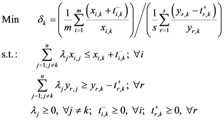
Stage 2―Classification of DMUs: For each DMU, solve the following slacks-based measure (SBM) model (Tone, [11] ):

(1)

where denotes the number of DMUs, is the number of inputs, is the number of outputs, is the amount of input used by, is the amount of output produced by, is the weight assigned to in constructing its ideal benchmark, and and are slack variables associated with the first and the second sets of constraints, respectively. If the optimal objective function value, then is classified as efficient. If, is classified as inefficient. Note that Model 1 above is solved as it is if Stage 1 reveals that the CRS conditions hold; otherwise, one would have to impose one of the following additional constraints depending on whether VRS, IRS, or DRS conditions prevail, respectively:

(2)

Stage 3―Break Efficiency Ties: For each efficient, solve the following slacks-based super-efficiency DEA model―first proposed by Tone [27] :

(3)

where (respectively,) denotes the amount by which input (respectively, output) of the efficient should be increased (respectively, decreased) to reach the frontier constructed by the remaining DMUs. Note that Model 2 above is solved as it is if Stage 1 reveals that the CRS conditions hold; otherwise, one would have to impose an additional constraint from amongst (2) as outlined in Stage 2. Use the super-efficiency scores to rank order the efficient DMUs.

At this stage, it is worth mentioning that unlike radial super-efficiency DEA models (e.g., Anderson and Peterson [8] ), slacks-based super-efficiency models are always feasible (Tone [27] ; Du et al. [28] ). Note that Tone [27] and Du et al. [28] slacks-based super-efficiency models are identical with respect to their constraints in that one could be obtained from the other using a simple variable transformation. Note, however, that in applications where positive input and output data is a requirement, Du et al. [28] provide a variant of the model solved in stage 3 to accommodate this situation. In the next section, we shall use the above described methodology to rank order competing crude oil prices’ volatility forecasting models.

4. Empirical Investigation and Results

In this paper, we focus on WTI crude oil daily spot prices and our data covers the period ranging from January 1986 to May 2010 resulting in a total of 6157 observations―note that the choice of this period is motivated by comparison purposes with the results obtained by Xu and Ouenniche [1] .

As crude oil prices are level non-stationary, in the literature there is a tendency to study their level stationary equivalent; namely, returns. We compute daily WTI crude oil returns as follows:

(4)

where denotes WTI crude oil price on day―obviously these returns are, which was confirmed by Augmented Dickey-Fuller test, Phillips-Peron test, and Kwiatkowski-Phillips-Schmidt-Shin test. Volatility of crude oil returns could be measured in several ways. In fact, one could measure volatility over the time unit under consideration (e.g., day, week, or month) by any dispersion measure such as variance or standard deviation, mean absolute deviation, or range of returns―as long as the relevant data is available (e.g., intra-day returns for daily volatility); however, such measures are affected by outliers; therefore, their use is only appropriate when the distribution of returns is symmetric or normal. In addition, when volatility is computed using high frequency data (e.g., intra-day returns), realized volatility could end up being very noisy as a result of market microstructure effects such as non-synchronous trading, discrete price observations, intraday periodic volatility patterns, and bid-ask bounce. Since crude oil daily returns are not normally distributed―as confirmed by the Jarque-Bera test of normality, in this paper we opt for an alternative approach to modelling daily volatility that consists of using daily squared returns as a proxy (e.g. Sadorsky [5] ; Agnolucci [6] ; Kang et al. [12] ). One however should be aware that squared daily returns provide a noisy proxy, but remains an unbiased estimator (Andersen and Bollerslev [29] ). The same tests performed on returns were performed on squared returns and results revealed that such volatility proxy series is also level-stationary and auto-correlated.

Within the proposed DEA framework, volatility forecasting models are used as DMUs, measures of biasedness and goodness-of-fit are used as input, whereas measures of correct sign are used as output―see Xu and Ouenniche [1] for descriptions of forecasting models and performance measures. Note that the choice of our inputs (respectively, outputs) is motivated by the principle of “the less the better” (respectively, “the more the better”). Note also that we have chosen to consider several measures for each criterion to find out about the robustness of multidimensional rankings with respect to different measures.

Table 1 provides the unidimensional rankings of fourteen forecasting models of crude oil returns volatility based on nine measures of three criteria; namely, goodness-of-fit, biasedness and correct sign―this is a typical output presented by most existing forecasting studies (Sadorsky [4] [5] ; Agnolucci [6] ; Marzo and Zagaglia [7] ). These unidimensional rankings are devised as follows: models are ranked from best to worst using the relevant measure of each of the criteria under consideration. Notice that different criteria led to different unidimensional rankings, which provides additional evidence of the problem resulting from the use of a unidimensional approach in a multicriteria setting as discussed in Section 1. For example, CGARCH (1, 1) outperforms SMA20 on measures of goodness-of-fit based on squared errors, whereas SMA20 performs better with respect to the biasedness criterion, as measured by both Mean Error (ME) and Mean Volatility-Adjusted or Scaled Errors (MVolScE), and with respect to the correct sign criterion, as measured by Percentage of correct direction change predictions (PCDCP). In order to remedy to these mixed performance results, one would need a single ranking that takes account of multiple criteria, which we provide using the proposed DEA framework.

Table 2 summarizes the multidimensional rankings of fourteen competing volatility forecasting models for several combinations of performance measures, where the models are ranked from best to worst based on the corresponding super-efficiency scores obtained using both input-oriented and output-oriented radial super-efficiency DEA models. Notice that, under VRS conditions, the rankings of input-oriented analysis and outputoriented analysis are different, on one hand, and the rankings of output-oriented analysis show more infeasibilities and/or ties, on the other hand. As to Table 3, it summarizes the multidimensional rankings of volatility forecasting models for several combinations of performance measures, where the models are ranked in descending order of the corresponding super-efficiency scores obtained using an orientation-free non-radial super-efficiency DEA model―see Section 3.

Table 2, Table 3 reveal that the rankings of forecasting models obtained by input-oriented super-efficiency DEA analysis, output-oriented super-efficiency DEA analysis, and orientation-free super-efficiency DEA analysis are different. Such differences are mainly due to the fact that input-oriented analysis minimizes inputs for fixed amounts of output and output-oriented analysis maximizes outputs for fixed amounts of input, whereas orientation-free analysis optimizes both inputs and outputs simultaneously. In addition, input-oriented super ef

References

- Xu, B. and Ouenniche, J. (2012) A Data Envelopment Analysis-Based Framework for the Relative Performance Evaluation of Competing Crude Oil Prices’ Volatility Forecasting Models. Energy Economics, 34, 576-583.http://dx.doi.org/10.1016/j.eneco.2011.12.005
- Hamilton, J.D. (2008) Oil and the Macroeconomy. In: Durlauf, S. and Blume, L., Eds., The New Palgrave Dictionary of Economics, Palgrave MacMillan. http://dx.doi.org/10.1057/9780230226203.1215
- Kilian, L. (2008) The Economic Effects of Energy Price Shocks. Journal of Economic Literature, 46, 871-909.http://dx.doi.org/10.1257/jel.46.4.871
- Sadorsky, P. (2005) Stochastic Volatility Forecasting and Risk Management. Applied Financial Economics, 15, 121-135. http://dx.doi.org/10.1080/0960310042000299926
- Sadorsky, P. (2006). Modelling and forecasting petroleum futures volatility. Energy Economics, 28, 467-488.http://dx.doi.org/10.1016/j.eneco.2006.04.005
- Agnolucci, P. (2009) Volatility in Crude Oil Futures: A Comparison of the Predictive Ability of GARCH and Implied Volatility Models. Energy Economics, 31, 316-321. http://dx.doi.org/10.1016/j.eneco.2008.11.001
- Marzo, M. and Zagaglia, P. (2010) Volatility Forecasting for Crude Oil Futures. Applied Economics Letter, 17, 1587-1599. http://dx.doi.org/10.1080/13504850903084996
- Andersen, P. and Petersen, N.C. (1993) A Procedure for Ranking Efficient Units in Data Envelopment Analysis. Management Science, 39, 1261-1294. http://dx.doi.org/10.1287/mnsc.39.10.1261
- Banker, R.D., Charnes, A. and Cooper, W.W. (1984) Models for the Estimation of Technical and Scale Inefficiencies in Data Envelopment Analysis. Management Science, 30, 1078-1092. http://dx.doi.org/10.1287/mnsc.30.9.1078
- Charnes, A., Cooper, W.W. and Rhodes, E. (1978) Measuring the Efficiency of Decision Making Units. European Journal of Operational Research, 2, 429-444. http://dx.doi.org/10.1016/0377-2217(78)90138-8
- Tone, K. (2001) A Slacks-Based Measure of Efficiency in Data Envelopment Analysis. European Journal of Operational Research, 130, 498-509. http://dx.doi.org/10.1016/S0377-2217(99)00407-5
- Kang, S.H., Kang, S.M. and Yoon, S.M. (2009) Forecasting Volatility of Crude Oil Markets. Energy Economics, 31, 119-125. http://dx.doi.org/10.1016/j.eneco.2008.09.006
- Wang, Y.D. and Wu, C.F. (2012) Forecasting Energy Market Volatility Using GARCH Models: Can Multivariate Models Beat Univariate Models? Energy Economics, 34, 2167-2181. http://dx.doi.org/10.1016/j.eneco.2012.03.010
- Day, T.E. and Lewis, C.M. (1993). Forecasting Futures Market Volatility. The Journal of Derivatives, 1, 33-50.http://dx.doi.org/10.3905/jod.1993.407876
- Fong, W.M. and See, K.H. (2002) A Markov Switching Model of the Conditional Volatility of Crude Oil Futures Prices. Energy Economics, 24, 71-95. http://dx.doi.org/10.1016/S0140-9883(01)00087-1
- Nomikos, N.K. and Pouliasis, P.K. (2011) Forecasting Petroleum Futures Markets Volatility: The Role of Regimes and Market Conditions. Energy Economics, 33, 321-337. http://dx.doi.org/10.1016/j.eneco.2010.11.013
- Ghysels, E., Harvey, A. and Renault, E. (1996) Stochastic Volatility. In: Maddala, G.S. and Rao, C.R., Eds., Handbook of Statistics 14: Statistical Methods in Finance, Elsevier Science, Amsterdam.
- Poon, S.H. and Granger, C.W.J. (2003) Forecasting Financial Market Volatility: A Review. Journal of Economic Literature, 41, 478-539. http://dx.doi.org/10.1257/jel.41.2.478
- Charnes, A. and Cooper, W.W. (1962) Programming with Linear Fractional Functionals. Naval Research Logistics Quarterly, 15, 333-334.
- Johnson, A.L. and Ruggiero, J. (2012) Nonparametric Measurement of Productivity and Efficiency in Education. Annals of Operations Research, 194, 1-14. http://dx.doi.org/10.1007/s10479-011-0880-9
- Korhonen, P.J. and Syrjanen, M.J. (2003) Evaluation of Cost Efficiency in Finnish Electricity Distribution. Annals of Operations Research, 121, 105-122. http://dx.doi.org/10.1023/A:1023355202795
- Ozcan, Y.A., Lins, M.E., Lobo, M.S.C., da Silva, A.C.M., Fiszman, R. and Pereira, B.B. (2010) Evaluating the Performance of Brazilian University Hospitals. Annals of Operations Research, 178, 247-261.http://dx.doi.org/10.1007/s10479-009-0528-1
- Seiford, L.M. (1997) A Bibliography for Data Envelopment Analysis (1978-1996). Annals of Operations Research, 73, 393-438. http://dx.doi.org/10.1023/A:1018949800069
- Cooper, W.W., Seiford, L.M. and Tone, K. (2007) Introduction to Data Envelopment Analysis and Its Uses: With DEA-Solver Software and References. 2nd Edition, Springer, New York.
- Liu, J.S., Lu, L.Y., Lu, W.M. and Lin, B.J. (2013) A Survey of DEA Applications. Omega, 41, 893-902.http://dx.doi.org/10.1016/j.omega.2012.11.004
- Banker, R.D., Cooper, W.W., Seiford, L.M., Thrall, R.M. and Zhu, J. (2004) Returns to Scale in Different DEA Models. European Journal of Operational Research, 154, 345-362. http://dx.doi.org/10.1016/S0377-2217(03)00174-7
- Tone, K. (2002) A Slacks-Based Measure of Super-Efficiency in Data Envelopment Analysis. European Journal of Operational Research, 143, 32-41. http://dx.doi.org/10.1016/S0377-2217(01)00324-1
- Du, J., Liang, L. and Zhu, J. (2010) A Slacks-Based Measure of Super-Efficiency in Data Envelopment Analysis: A Comment. European Journal of Operational Research, 204, 694-697. http://dx.doi.org/10.1016/j.ejor.2009.12.007
- Andersen, T.G. and Bollerslev, T. (1998) Answering the Skeptics: Yes, Standard Volatility Models Do Provide Accurate Forecasts. International Economic Review, 39, 885-905. http://dx.doi.org/10.2307/2527343
NOTES
*Corresponding author.