Abstract

In wireless sensor networks, sensor nodes collect local data and transfer to the base station often relayed by other nodes. If deploying sensor nodes evenly, sensor nodes nearer to the base station will consume more energy and use up their energy faster that reduces system lifetime. By analyzing energy consumption, a density formula of deploying nodes is proposed. The ratio of whole energy of sensor nodes to energy consumption speed of sensor nodes in every area can get consistent if deploying nodes by the density formula, therefore system lifetime is prolonged. Analysis and simulation results show that when communication dominates whole energy consumption and the monitored region is big compared with radio range of sensor node, system lifetime under this scheme can be 3R/(2t) times of that under deploying nodes evenly, where R is radius of the monitored region and t is radio range of sensor node.

1.Introduction

Recently, wireless sensor networks composed of large sensor nodes come to realize [1-4]. Sensor nodes have very limited processing and communication capabilities. Sensor networks are multi-hop and sensor nodes play a dual role as both data generators and routers [5]. Energy is identified as one of the most crucial resources in sensor networks dual to the difficulty of recharging batteries of thousands of devices in remote or hostile environments [6-8]. Researches show that energy consumption of sensor node is dominated by communication [4,9].

In a typical sensor network, there is a base station in the network. Sensor nodes sense environment, collect sensor reading, process the data and then forward the information to the base station. An example of such applications is habitat monitored [10]. Sensor nodes are deployed in the habitat and the base station collects data from sensor nodes. So information of the habitat can be achieved from the base station.

Because remote sensor nodes transferring data to the base station needs some close nodes to relay, data stream density nearer to the base station is bigger. If sensor nodes are deployed evenly, nodes nearer to the base station will consume more energy. If close nodes use up their energy, other nodes can’t transfer their data to the base station and system lifetime of sensor network is over.

Presently, there’s few research about deploying nodes with the purpose of prolonging system lifetime. Most researches assumed that sensor nodes are deployed evenly scattered by airplane or other tools in the monitored region [11,12]. So system lifetime of the sensor network can’t be long. [13] researched data stream in wireless sensor network and showed that data streams of different areas aren’t balancing. Data stream of middle area is dense while data stream of boundary area is sparse. This paper determinates rational scheme of deploying nodes by researching energy consumption in different areas to prolong system lifetime.

The remainder of this paper is organized as follows. In section 2, assumptions and base model are given. Section 3 describes how to deploy nodes in wireless sensor networks. Section 4 presents some theoretic analysis and section 5 presents a comparative performance evaluation using simulation. This paper concludes with section 6.

2. Assumptions and Base Model

This section presents the basic model of the sensor network that this paper targets. The network model makes the following assumption:

-    Wireless sensor network is large-scale. There are many sensor nodes and a base station in the network. Monitored region of the sensor network is a circle which radius is R. The base station is located in the center of the circle.

-    Sensor nodes are homology. Initial energy of sensor node is e.

-    Each sensor node senses environment and transfers local information to the base station. Events occur evenly in the monitored region. Data generating speed is λ per unit area.

-    Sensor nodes communicate with the base station by delivering data across multiple hops. Radio range of sensor node is t.

-    Energy consumption of sensor nodes transmitting unit data and receiving unit data is T and E respectively.

-    Energy consumption not caused by communication is evenly distributed in the monitored region. Other energy consumption speed per unit area is W.

In above, we assume that the monitored region is a circle for the sake of analyzing easily. System lifetime is mostly optimized when the base station is located in the center.

3.Scheme of Deploying Nodes

In this section, we will deduce a density formula of deploying nodes that will prolong system lifetime of wireless sensor networks.

In wireless sensor networks, the ratio of whole energy of sensor nodes to energy consumption speed of sensor nodes in every area should be consistent. Thus more sensor nodes will be deployed in area where energy is consumed sooner. As a whole, sensor nodes in different areas will tend to use up energy at the same time. Therefore system lifetime gets prolonged furthest.

Because we have assumed that the monitored region is center symmetry, node density should be only relational with distance to the base station. We denote ρ(r) as node density of point that is r far from the base station.

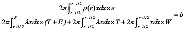
Next we analyze energy consumption in area B in Figure 1. Area B is a ring centered at the base station that inner radius is r-t/2 and outer radius is r+t/2. Because radio range of sensor node is t, sensor nodes that are farther from the base station than r+t/2 (i.e. sensor nodes outside area B) transferring data to the base station needs some node in area B to relay.

Data generating speed outside area B is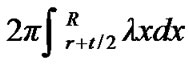. Energy consumption speed of sensor nodes in area B

relaying data generated outside area B is. Data generating speed in area B is. Energy consumption speed of sensor nodes in area B transmitting data generated in area B is. Other energy consumption speed in area A is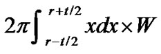. So energy consumption of sensor nodes in area B is

.

The number of sensor nodes in area B is. So the whole energy of sensor nodes in area B is.

The ratio of whole energy of sensor nodes to energy consumption speed of sensor nodes in area B should be a constant. So following condition is satisfied:

where b is a constant.

Because node density of each point in area B is almost equal. So we approximately choose ρ(r) as average node density of area B. i.e..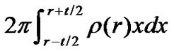

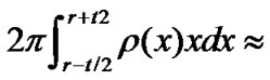So we can get:

From the above formula, we can deduce:

.

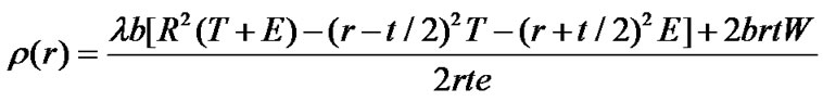When r/t large, we have r-t/2≈r, r+t/2≈r. So we get:

, where,.

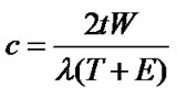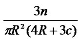
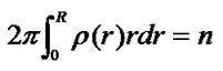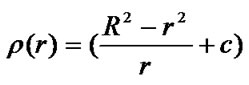
Assume that the number of all sensor nodes is n, then. We can deduce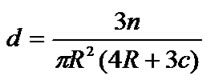. So we can obtain node density of point that is r far from the base station:

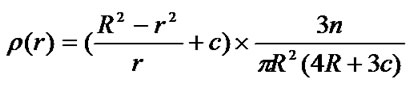, where.

From above density formula, node density of close area is bigger than that of remote area. It is consistent with our expectation.

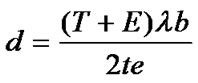
ρ(r) consists of two parts: and c, where is reverse with distance to the base station and c is a constant ?/span>independent of distance to the base station. In the formula of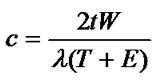, λ(T+E) is energy consumption speed of sensor nodes transmitting and receiving data and W is other energy consumption speed. If the proportion of other energy consumption speed is bigger, c is bigger and node densities of the monitored region tend to be more even. Otherwise node densities of the monitored region tend to be more uneven. This is because other energy consumption speeds in different areas are close while energy consumption speeds of sensor nodes transmitting and receiving data in different areas are different.

4.Analysis of System Lifetime

In this section, we will analyze system lifetime under deploying nodes by the density formula deduced in last section compared with deploying nodes evenly in wireless sensor network.

First analyze system lifetime under deploying nodes by the density formula . Because in this case the ratio of whole energy of sensor nodes to energy consumption speed of sensor nodes in every area is consistent, sensor nodes in every area tend to use up their energy at the same time. Then system lifetime approximates the ratio of whole energy of sensor nodes to energy consumption speed of sensor nodes in some area. Therefore we can only analyze system lifetime of sensor nodes in area C which is less than t far from the base station.

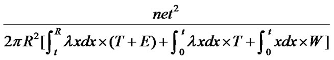
Energy consumption speed of sensor nodes in area C is. Whole energy of sensor nodes in area C is =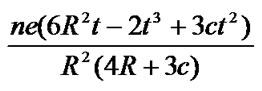. So system lifetime is:

.

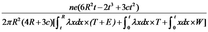
Next let抯 analyze system lifetime under deploying nodes evenly. Sensor nodes outside area C transferring data to the base station needs some node in area C to relay. Because sensor nodes are deployed evenly, energy consumption speed of sensor nodes in area C is fastest. Therefore sensor nodes in area C will use up their energy earliest. When sensor nodes in area C use up their energy, the base station can抰 receive any data from the sensor network and system lifetime is over. So system lifetime approximates the ratio of whole energy of sensor nodes to energy consumption speed of sensor nodes in area C also.

Energy consumption speed of sensor nodes in area C is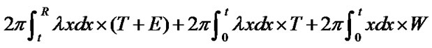. Whole energy of sensor nodes in area C is. So system lifetime is:

.

The ratio of system lifetime under deploying nodes by the density formula to that under deploying nodes evenly is:

where t and c are fixed values.

From the above ratio, we can see system lifetime under deploying nodes by the density formula is long than that under deploying nodes evenly. When other energy consumption is little and the monitored region is big, i.e. c≈0 and R?i style='mso-bidi-font-style:normal'>t, the ratio approximates to 3R/(2t). Because t is a fixed value, the ratio is bigger when the monitored region is larger.

5.Simulation

In this section, we compare system lifetime under deploying nodes by the density formula proposed by this paper with deploying nodes evenly by simulation. We adopt ns-2.28 simulator [14] as experiment platform. We use the following model for our simulation study:

-    MAC protocol is 802.11 DCF.

-    Radio bandwidth is 1 Mbps.

-    Radio range is 50 m.

-    Initial power of sensor node is 10000 J.

-    Sensor node’s sending and receiving power are 0.660 W and 0.395 W respectively.

-    The size of packet is 64 B.

-    Other energy consumption of sensor node is 0.

-    The occurring of event in the monitored region satisfies Poisson distribution. The speed of event occurring in area is 0.01 m^-2s^-1.

-    Sensing data of one event has 10 packets averagely.

We simulate under various sizes of the monitored region. Choose radiuses of the monitored region be 200 m, 400 m, 600 m, 800 m, and 1000 m. Fix average node density of the whole monitored area be 1/(400π) m^-2. So the numbers of sensor nodes in various monitored regions are 100, 400, 900, 1600 and 2500 respectively. We choose system lifetime as the time from beginning to when average ratio of event being successfully monitored by the base station is under a threshold of 90%. Observe system lifetime under various simulation conditions. In order to make results more precise, we simulate 10 times for each simulation condition and choose average value.

Table 1 shows system lifetime under various conditions. R denotes radius of the monitored region. t denotes radio range. n denotes the number of sensor nodes. α denotes system lifetime under deploying nodes by the density formula proposed by this paper. β denotes system lifetime under deploying nodes evenly. The ratio of system lifetimes under these two schemes is near to 3R/2t. It’s consistent with analysis result in section 4. Figure 2 shows comparison of system lifetimes under these two schemes. System lifetime under deploying nodes by the density formula proposed by this paper is much longer than deploying nodes evenly.

6.Conclusions

This paper deduces the density formula 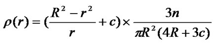of deploying nodes in wireless sensor networks by analyzing energy consumption speeds in different areas. The ratio of whole energy of sensor nodes to energy consumption speed of sensor nodes in every area can get consistent if deploying nodes by the density formula. Then we analyze system lifetime under this scheme of deploying nodes. When communication dominates whole energy consumption and the monitored region is big compared with radio range of sensor node, system lifetime under this scheme can be 3R/(2t) times of that under deploying nodes evenly, where R is radius of the monitored region and t is radio range of sensor node. Finally simulation results validate this conclusion.

7. Acknowledgement

The research was jointly supported by research grants from Natural Science Foundation of China under project number 60602066 and 60773203, grant from Guangdong Natural Science Foundation under project number 5010494. The work has also got support from Foundation of Shenzhen City under project number QK200601. Corresponding author: Ke-Zhong Lu (kzlu@szu.edu.cn).

8.References

[1]       I. F. Akyildiz, W. Su, Y. Sankarasubramaniam, and E. Cayirci, "Wireless sensor networks: a survey," Computer Networks, 38(4), pp. 393-422, 2002.

[2]       S. Brown and C.J. Sreenan, "A new model for updating software in wireless sensor networks,"IEEE Network, 20(6), pp. 42-47, 2006.

[3]       L. Cui, H. L. Ju, Y. Miao, T. P. Li, W. Liu, and Z. Zhao,"Overview of wireless sensor networks,"Journal of Computer Research and Development, 42(1), pp. 163-174, 2005.

[4]       J. M. Kahn, R. H. Katz, and K. S. J. Pister,"Next century challenges: mobile networking for smart dust," in Proceedings of the 5th Annual ACM/IEEE International Conference on Mobile Computing and Networking, pp. 263-270, 1999.

[5]       H. S. Kim, T. F. Abdelzaher, and W. H. Kwon,"Minimum-energy asynchronous dissemination to mobile sinks in wireless sensor networks," in Proceedings of the 1st International Conference on Embedded Networked Sensor Systems, pp. 193-204, 2003.

[6]       Y. Yang, V. K. Prasanna, and B. Krishnamachari, "Energy minimization for real-time data gathering in wireless sensor networks,"IEEE Transactions on Wireless Communications, 5(11), pp. 3087-3096, 2006.

[7]       H. Kwon, T. H. Kim, S. Choi, and B. G. Lee,"A cross-layer strategy for energy-efficient reliable delivery in wireless sensor networks,"IEEE Transactions on Wireless Communications, 5(12), pp. 3689-3699, 2006.

[8]       Y. W. Hong and A. Scaglione, "Energy-efficient broadcasting with cooperative transmissions in wireless sensor networks,"IEEE Transactions on Wireless Communications, 5(10), pp. 2844-2855, 2006.

[9]       Y. Yu, V. K Prasanna, and B. Krishnamachari, "Energy minimization for real-time data gathering in wireless sensor networks,"IEEE Transactions on Wireless Communications, 5(11), pp. 3087-3096, 2006.

[10]    A. Mainwaring, J. Polastre, R. Szewczyk, D. Culler, and J. Anderson, "Wireless sensor networks for habitat monitored," in First ACM Workshop on Wireless Sensor Networks and Applications, pp. 88-97, 2002.

[11]    J. Chen, Y. Guan, and U. Pooch, "A spatial-based multi-resolution data dissemination scheme for wireless sensor networks,"in the 5th IEEE International Workshop on Algorithms for Wireless, Mobile, Ad Hoc and Sensor Networks, 2005.

[12]    J. Chen, Y. Guan, and U. Pooch, "An efficient data dissemination method in wireless sensor networks," in the IEEE Global Telecommunications Conference, 2004.

[13]    U. Bilstrup, K Sjoberg, B. Svensson, and P. A. Wiberg, "Capacity limitations in wireless sensor networks,"in Proceedings of IEEE International Conference on Emerging Technologies and Factory Automation, pp. 529-536, 2003.

[14]   "Network Simulator", http://www.isi.edu/nsnam/ns.