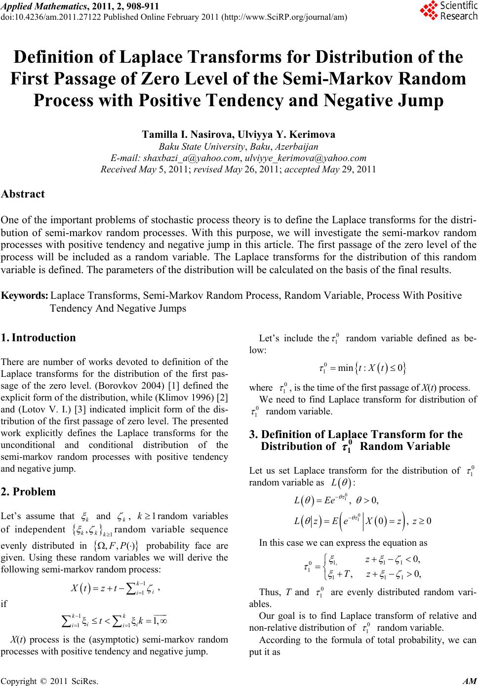
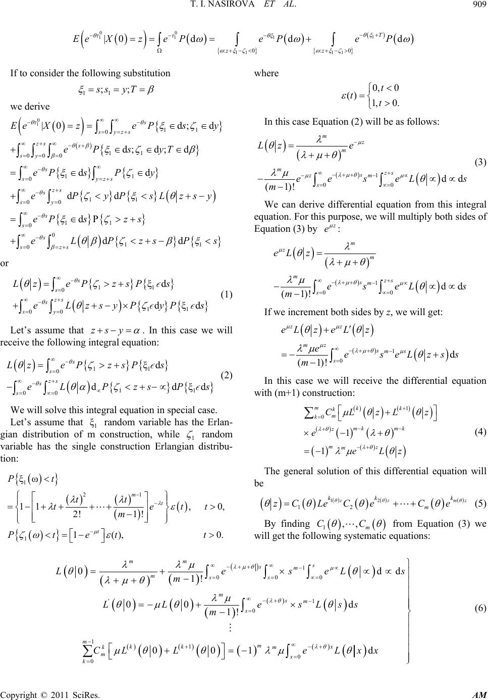
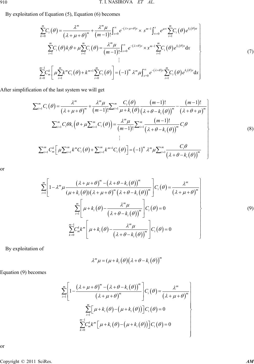
Applied Mathematics, 2011, 2, 908-911
doi:10.4236/am.2011.27122 Published Online February 2011 (http://www.SciRP.org/journal/am)
Definition of Laplace Transforms for Distribution of the
First Passage of Z er o Lev el o f th e Semi-Mark o v Ra nd om
Process with Positive Tendency and Negative Jump
Tamilla I. Nasirova, Ulviyya Y. Kerimova
Baku State University, Baku, Azerbaijan
Received May 5, 2011; revised May 26, 2011; accepted May 29, 2011
Abstract
One of the important problems of stochastic process theory is to define the Laplace transforms for the distri-
bution of semi-markov random processes. With this purpose, we will investigate the semi-markov random
processes with positive tendency and negative jump in this article. The first passage of the zero level of the
process will be included as a random variable. The Laplace transforms for the distribution of this random
variable is defined. The parameters of the distribution will be calculated on the basis of the final results.
Keywords: Laplace Transforms, Semi-Markov Random Process, Random Variable, Process With Positive
Tendency And Negative Jumps
1. Introduction
There are number of works devoted to definition of the
Laplace transforms for the distribution of the first pas-
sage of the zero level. (Borovkov 2004) [1] defined the
explicit form of the distribution, while (Klimov 1996) [2]
and (Lotov V. I.) [3] indicated implicit form of the dis-
tribution of the first passage of zero level. The presented
work explicitly defines the Laplace transforms for the
unconditional and conditional distribution of the
semi-markov random processes with positive tendency
and negative jump.
2. Problem
Let’s assume that k

and k

, random variables 1k
of independent

random variable sequence

1
,
kk
k


evenly distributed in

probability face are
given. Using these random variables we will derive the
following semi-markov random process:

,,()FP

1
1
k
i
i
Xtz t





,
if
1
11
ξξ1,
kk
ii
ii
tk


 


X(t) process is the (asymptotic) semi-markov random
processes with positive tendency and negative jump.
Let’s include the0
1

random variable defined as be-
low:



0
1min :0tXt



where 0
1

, is the time of the first passage of X(t) process.
We need to find Laplace transform for distribution of
0
1

random variable.
3. Definition of Laplace Transform for the
Distribution of 0
1

Random Variable
Let us set Laplace transform for the distribution of 0
1

random variable as


L

:





0
 1
0
1
0,
0, 0
, LEe
LzEe Xzz







1
In this case we can express the equation as
1,1 1 0
1
11
0,
, 0,
z
Tz








Thus, T and 0
1

are evenly distributed random vari-
ables.
Our goal is to find Laplace transform of relative and
non-relative distribution of 0
1

random variable.
According to the formula of total probability, we can
put it as

T. I. NASIROVA ET AL.909


 




00 1
11 1
11 11
:0 :0
|0 ddd
T
zz
EeXze PePeP

 




 
 
 

If to consider the following substitution
11
;;ss yT

 
we derive





 



 


0
1
11
0
11
00 0
11
0
11
00
11
0
11
0
|0d;d
d;d; d
dd
dd
dP
dd
s
syzs
zs s
sy
s
syzs
zs
s
sy
s
s
s
s
EeXze Psy
ePsyT
ePs Py
ePyPsLzsy
eP szs
eLPzsP
 








 



  





 










 

 








0
zs


s


or




11
0
11
00
ξd
dξd
s
s
zs
s
sy
LzeP zsP s
eLzsyPyP
















s
(1)
Let’s assume that zsy

 . In this case we will
receive the following integral equation:




11
0
1
00
ξd
ddξd
s
s
zs
s
s
LzePzsP s
eL PzsP



 













1
s
(2)
We will solve this integral equation in special case.
Let’s assume that 1 random variable has the Erlan-
gian distribution of m construction, while 1
ξ

random
variable has the single construction Erlangian distribu-
tion:




 
 
 
1
21
1
ξω
11, 0,
2!1 !
1(), 0.
m
t
t
Pt
tt
tet
m
Ptet t




 







  







 


where
0, 0
() 1, 0.
t
tt





In this case Equation (2) will be as follows:




1
00
dd
(1)!
mz
m
mzs
s
zm
s
Lz e
ee se
mL





 







 s
(3)
We can derive differential equation from this integral
equation. For this purpose, we will multiply both sides of
Equation (3) by
z
e

:




1
00
dd
(1)!
m
zm
mzs
sm
s
eL z
eseL
m

 


 





 s
If we increment both sides by z, we will get:






1
0d
(1)!
zz
mz sms
s
eLzeLz
eeseLzs
m



 




 
s
In this case we will receive the differential equation
with (m+1) construction:







 



1
0
1
1
mkk
k
m
k
mk mk
z
mz
m
CL zLz
e
eLz


 

 













(4)
The general solution of this differential equation will
be
t








12
12
z
zm
kk
m
zC LeCeCe

  z
k

(5)
By finding


,,
m
CC

1

  from Equation (3) we
will get the following systematic equations:





 










1
000
' 1
0
11
0
0
0 d
1!
00 d
1!
001 d
mm s
sm
mss
msm
s
mm
kk x
km
mx
k
Lese
m
LL esLss
m
CLLe Lxx
 







 

 

 









 


 




 

 





dLs 
(6)

T. I. NASIROVA ET AL. 910
By exploitation of Equation (5), Equation (6) becomes
 




 







1
00
0 1
1
0
11 1
1
1
0
01 01
1!
d
1!
1d
i
i
i
mm
m m
s
sk
m
i i
ms
k i
m
mm m
xkx
m
ii ii
s
ii i
mm mm
mxkx
km mm
mi ii
x
ki ii
Cese
m
CkCex Cex
m
CkCkCeCe


 
 





 
 

 
 

 



 

 


 







 

 














Ce
x
(7)
After simplification of the last system we will get
 






 





 


 

11
11 1
1
11 11
1! 1!
1!
1!
1!
1
mm
mm
i
imm
ii
ii
m
mm m
ii ii
m
ii i
i
m mm mm
km mmi
mi im
ii ii
i
Cm m
Cmk
k
m
Ck CC
mk
C
CkC kCk



 


 
 

 


 

 

 


 
 


 
 





 
 

 
 

m


(8)
or
  
 
 
 


 


1
1
1
0
1
()
0
0
m
mm
mi
mi
mm
m
iii
m
m
ii
m
ii
m
mkm
mi i
m
ki
kC
kk
kC
k
Ck kC
k
 
 


 


 







 












 

 






 








(9)
By exploitation of
 

(m
mii
kk   
Equation (9) becomes
  
  
   
 


1
1
1
0
1
0
0
m
mm
mii
mm
i
m
iii
i
mkm
mi ii
k
kC
kkC
Ckkk C
 

 
 
 






 





 





 




 








or

T. I. NASIROVA ET AL. 911
 


1
1
1
00
00
mmm
ii
i
m
i
i
m
i
i
kC
C
C

 






 



 




 





(10)
Thus, (9) is a linear dependence equation system, as
 
 
23
1
1
0
m
m
m
CC C
Ck
 

 





Then the general solution of integral Equation (3) will
be as follows:
 



11
1
1
z
z
m
kk
m
LzC ee
k


  


This expression is the Laplace transform for relative
distribution of 0
1

random variable. Then, we will need
to find

L

. In accordance with formula of total prob-
ability,
   
z0
LzdPX0L




z
and as the distribution of X(0) and

1


random
variables are same,
 

 






 
1
1
1
1
z0
1
1z0
11
z0
1
1
dP 0
d
1!
d
1!
z
z
k
m
kmz
mkz
m
m
m
LCeXz
Ce ze
m
Cezz
m
C
k














 












z

Therefore,
  
1
1
m
m
LC
k







This expression is the Laplace transform for non-rela-
tive distribution of 0
1

random variable.
Respectively, we will get the following characteristics
for ߣm > ߤ:




 

 


  


 











0
1
32 3
2
2
3
32
2
0
12
2
3
2
2
32
2
0
1
0
123
0
3
02
1
(
3
00
2
1
1
z
1( )
z
m
EL m
mm m
Lm
m
mm
m
mm
DL Lm
m
m
mmm m
mm
mz
Em
mm mz
m
Dmm

 












 

 



 


 








 









4. Conclusions
In this article we have defined Laplace transforms for
relative and non-relative distribution of the first passage
of zero level of semi-markov random process with posi-
tive tendency and negative jump.
5. References
[1] A. A. Borovkov, “On the Asymptotic Behavior of the
Distributions of First-Passage,” Mathematics and Stati-
stics, Vol. 75, No. 1, 2004, pp. 24-39.
doi:10.1023/B:MATN.0000015019.37128.cb
[2] V. I. Lotov, “On the Asymptotics of the Distributions in
Two-Sided Boundary Problems for Random Walks
Defined on a Markov Chain,” Siberian Advances in
Mathematics, Vol. 1, No. 3, 1991, pp. 26-51.
[3] G. P. Klimov, “Stochastic Queuening Systems,” Nauka,
Moscow, 1966.
[4] T. I. Nasirova and R. I. Sadikova, “Laplace Trans-
formation of the Distribution of the Time of System
Sojourns within a Band,” Automatic Control and Computer
Sciences, Vol. 43, No. 4, pp. 190-194.
doi:10.3103/S014641160904004X