Optics and Photonics Journal, 2015, 5, 247-259
Published Online July 2015 in SciRes. http://www.scirp.org/journal/opj
http://dx.doi.org/10.4236/opj.2015.57024
How to cite this paper: Hutchin, R.A. (2015) Toward a Local Theory of Light. Optics and Photonics Journal, 5, 247-259.
http://dx.doi.org/10.4236/opj.2015.57024
Toward a Local Theory of Light
Richard A. Hutchin
Optical Physics Company, Calabasas, CA, USA
Received 14 May 2015; accepted 28 July 2015; published 31 July 2015
Copyright © 2015 by author and Scientific Research Publishing Inc.
This work is licensed under the Creative Commons Attribution International License (CC BY).
http://creativecommons.org/licenses/by/4.0/
Abstract
Quantum mechanics is a probabilistic theory of the universe suggestive of a mean value theory
similar to thermodynamics prior to the introduction of the atomic theory. If QM will follow a simi-
lar path to thermodynamics, then a local deterministic theory must be developed which matches
QM predictions. There have been four tough barriers to a local theory of light, of which Bell’s
Theorem has been considered the ultimate barrier. The other three barriers are explaining spon-
taneous emission, the reflection of a small fraction of light at a dielectric interface and the splitting
action of a polarizer on polarized light (Malus’ Law). The challenge is that in a local theory of light,
everything must have a specific cause and effect. There can be nothing spontaneous or hidden.
Local solutions to all four of these barriers are presented in this paper, integrating results from
two previous papers and adding the solution paths to the third and fourth barriers as well, which
are nearly identical. A previous paper [1] used results from Einstein’s famous 1917 paper on sti-
mulated emission to provide a deterministic local model for spontaneous emission. A second pa-
per [2] showed that QM predictions in tests of Bell’s theorem could be matched with a local model
by modifying the definition of entanglement in a manner invisible to quantum mechanics. This
paper summarizes and extends those two results and then presents a deterministic model of ref-
lection from a dielectric interface and transmission of polarized light through a polarizer that both
match quantum mechanics. As the framework of a local theory of light emerges, it is not surprising
that we find corners of physics where small disagreements with quantum mechanics are predicted.
A new Bell type test is described in this paper which can distinguish the local from the nonlocal
theory, giving predictions that must disagree slightly but significantly with quantum mechanics. If
such experiments are proven to disagree with quantum mechanics, then the door to a local theory
of light will be opened.
Keywords
Entangled Photons, Bell’s Theorem, Local Theory of Light, Tests of Quantum Mechanics,
Spontaneous Emission, Malus’ Law, Reflection from a Dielectric

R. A. Hutchin
248
1. Introduction
Quantum mechanics has several key issues that remain unresolved after a hundred years of research. Consider
the collapse of a probability wave. What exactly is a probability wave and what makes it collapse? Even more
consider the complexity. There are an estimated 1078 - 1082 protons in the universe, first estimated by Eddington
[3], and we have estimated that the cumulative emission of all stars in the universe have launched over 1090
photons into space, most of which are still sailing through the cosmos. According to quantum mechanics, all
those photons do not really exist an ywhere or perhaps exist at all possib le places until the moment they collapse
to excite some electron or scatter off a particle. Given that most of those photons have been traveling for over a
billion light years, a usual dipole emission probability would have them anywhere in 1018 square light years,
which includes about 1062 possible positions (assuming each position is 1 × 1 um in size). Since almost all those
photons are currently tra veling through the cosmos, somehow the universe must keep track of 1062 × 1090 = 10152
positions of current photons updating them all every 1 um or so of propagation (every 3 × 10−15 sec) and com-
municating among all those positions so that when a photon does finally appear somewhere, the universe knows
which one it is and turns off its probability wave instantaneously at all other 1062 possible places that one photon
may have been. As a side note, this actually requires communicating back in time for all coordinate systems
since any place above the past light cone is “simultaneous” in some Lorentz frame.
A very complicated universe indeed is required by quantum mechanics, which must someday address the
question of how all that communication and tracking is accomplished.
Alternatively a local theor y says that each photon is always in a single locatio n, not somewhere in 1062 loca-
tions. Furthermore the photon would follow simple local laws on its propagation and interactions. Such a theory
would be 1062 time s less complicated than QM and would not require a hidden faster than light communication
system. This level of simplification of 1062 is like replacing 100,00 0 solar systems with a single p roton. Tha t is
the motivation to find a local theory of ligh t.
The structure of this paper is summarized here:
1) Overview of a prior paper [1] about the vacuum field, leading to a local and deterministic model of stimu-
lated emission.
2) A general discussion of several photonic clues from historical research.
3) The concept of photons being carried by the E & M River is presented with a covariant equation for photonic
flux.
4) A local theory of light is developed for how each photon decides to reflect or not at a dielectric transition,
such as a glass surface.
5) Application of the local theory of dielectric reflection to the problem of polarized light partially reflecting
and partially transmitting thr ough a polarizer (Malus’ Law).
6) An overview and extension of a prior paper [2] on Bell’s test for entangled photons, which provides a local
solution to entangled light that matches QM predictions.
7) A new test is derived for a local model of light from the work on Bell’s Test for entangled photons that will
measurably disagree with quantum mechanics under conditions of high quantum efficiency.
We respectfully caution the reader that exploring a relatively unknown area of science, such as a local theory
of light, inevitably leads to qualitative and as well as quantitative logic. We know from Bell’s theorem that a lo-
cal theory of light will be very different from classical E & M theory, so one can expect new paradigm’s anc-
hored in experiment and theory but also extrapolating to deeper levels not yet well explored. As always, experi-
ments will get the last word.
2. A New Physical Model for the Vacuum Field Based on Einstein’s Stimulated
Emission Theory [1] Overview
We can get insights into the photon by addressing the mystery of the vacuum field, sometimes called the zero-
point background. The vacuum E & M field comes from the 1 /2hν energy in the lowest state of a quantum os-
cillator, and it has the power spectral field density Ivac of Equation (1) when integrated over all directions (i.e. 4π
steradians) [4].
( )
( )
3
2
3
2
4π4πwatt cmHz
vac
hc h
Ic
ν
νλ = =
(1)

R. A. Hutchin
249
It was first proposed to be real and experimentally observ able by Hedrick Casimir, a Dutch scientist, in 1948
[5]. Subsequently, many experiments have confirmed that it has the expected field strength, which is measured
by the pressure exerted on two closely spaced reflecting surfaces [6]. For radiation longer than 10 nm wave-
length, this vacuum field density is about 1.8 × 1012 watt/cm2—a massive intensity equal to the entire power
generation of our world in 10 cm2. As a result of this huge electromagnetic intensity, the force from the pressure
of light on two parallel p lates a distance d apart is simply given by Equation (18), which computes to 18.85 psi
for a separation d = 10 nanometers. The minus sign means that the force is squeezing the plates together.
2
4
π
240
vac
c
Pd = −
(2)
Ref [6] summarizes past research in over 200 pages, validating the Casimir force well.
The biggest mystery of the vacuum field is that it has the E & M field strength of 2 terawatt/cm2 but does not
burn up everything as a normal E & M field of this strength would easily do. The conclusion is that the fields are
there as predicted (because we measure their pressure), but they must have something different about them that
prevents them from vaporizing everything.
The hint of this mysterious property we find in Clue 1, from Einstein’s paper on stimulated emission [7].
Clue 1: The spontaneous emission coefficient A21 has a simple physical relationship to the stimulated
emission coefficient B21 given by:
3
21
21 2decay
8π1 Bh
Ac
ν
τ
= =
(3)
In words, this result from Einstein’s paper says:
The spontaneous decay of any atom is identical to stimulated emission from a background spectral in-
tensity equal to twice the vacuum background (4πhν3/c2 in Equation (1)).
What is the meaning of Einstein ’s Equation (3), which has been mostly ignored? The logic we propose is the
following:
Hypothesis 1: Light comes in two independent and separable forms, up stimulating and down stimu-
lating, with the vacuum form being purely down stimulating.
This means that the vacuum field will have the field strength that is observed, but it has an additional quality
that makes it purely down stimulating and is thus unable to burn everything up. To explore what quality would
make an E & M field down stimulating only, we use another result from the same Einstein paper:
Clue 2: Blackbody light has, on average, an equal ability to cause an up transition (excitation) as it does
to cause a down transition (stimulated emission). Mathematically Einstein expressed this relationship as
B12 = B21, which means the cross-section for going from ground state 1 to excited state 2 equals the cross-
section for stimulating the transition from excited state 2 to excited state 1.
Focusing on Clue 2, we ask how can the real fields of blackbody emission be divided into two equal compo-
nents—one causing excitation and one causing stimulated emission? Our suggestion is to decompose all radia-
tion into e+iwt and e−iwt components, where e+iwt is up stimulating (excitation) and e−iwt is down stimulating (sti-
mulated emission). The sign convention is obviously arbitrary. When we look at power (defined here as mean
magnitude-squared since we are dealing with complex fields), we get that half the power of a real field goes into
the up-stimulating waveform and half into the down—an equal amount to each as required from Einstein’s paper
with B12 = B21.
For instance, a real E & M field of the form cos(kz − ct) will decompose into up and down stimulating terms
as shown in Equation (4). The mean-square-magnitude of the left side is 1/2, while the mean-square-magnitude
of each of the right terms is 1/4 . Note that the first term is purely e−iwt and the s e con d purely e+iwt.
( )
( )( )
ee
cos 22
i kzti kzt
kz t
ωω
ω
− −−
−= +
(4)
With this half and half power division into up and down stimulating fields, we modify Einstein’s result so that
the up-stimulating capability equ als 2B12 times the power in the up stimulating component, and the down stimu-
lating capability equals 2B21 times the power in the down stimulating component. Since half the power of the
real field goes into each up and down component, the final product is the same as he presented, only the inter-

R. A. Hutchin
250
pretati o n ha s c ha n ged.
Applying this result to th e vacuum field, which we model as pure ly down stimulating, we get that the ability
of the vacuum field to stimulate emission is 2B214πhc/λ3 = B218πhc/λ3 exactly as Einstein specified in Equation
(3).
Now we summarize this in a more complete set of hypotheses:
Hypothesis 1: Lig ht comes in two independent and separable forms, e+iwt and e−iwt, the first up stimulat-
ing and the second down stimulating.
Hypothesis 2: The vacuum field is purely of the e−iwt form, which produces the observed real component
of E & M fields, with out having any abilit y to up stimulate (ex c ite).
Hypothesis 3: All “spontaneous” emission is stimulated emission caused by the vacuum field.
While this research in the vacuum field was done for independent reasons, this result is important for a local
theory of light, where nothing can be “spontaneous”. In a local theory of light, everything must have a determi-
nistic physical cause. The vacuum field is the only ubiquitous random source in the universe and an excellent
candidate for producing the randomness we observe in other physical processes. For instance, this same vacuum
field will provide a local solution to ref lec tion a t a dielectric interface later in this paper .
3. Other Photonic Clues
Over the last hundred years we have accumulated thousands of experimental clues to the tru e nature of light. We
augment the first two clues above with a few of these that we have found especially useful in developing a local
theory of light.
Clue 3: When two detectors look at a single atomic source through a beamsplitter, no simultaneous
counts are observed.
This conclusion is commonly stated as: You can’t split a photon. Many scientists (including the author) have
tried clever ways to split one photon in two without success. The conclusion is that the photon must be a small
stable primal entity—wh at we might call a particle. The challen ge is then to integrate the p article nature of light
with the many interference phenomena we use every day.
Clue 4: In a cascade transition, the detection of the first transition initiates an exponential decay of the
counts from the second transition [8].
Clue 4 from Figure 3 of a 1974 paper by Clauser [8] has not been given much attention, but it provides im-
mediate and useful insight into the photon—the part of the E & M emission that causes excitation. He set up a
cascade transition in Calcium using nanosecond detectors to measure the emission time of each sequential pho-
ton. Then he plotted the time of detection of the second photon relative to the time of detection of the first ph o-
ton. He reported an exponentially decaying probability of detection for the second photon beginning exactly at
the moment of detection of the first photon. Since the emission of the second photon begins with full force as
soon as the first photon is emitted, we see that the photon emission comes at the time of the s tate transition. This
experimental result is so useful that we make its conclusion the 4th hypothesis of the local the ory and list it for-
mally:
Hypothesis 4: The photon is quite distinct and separable from the exponentially decaying E & M wave
that precedes it. It is emitted at the moment when one emitting state transitions to the next in the cascade.
Thus it appears to be at the end of the E & M emission from an excited state.
On top of these rather specific constr a ints, we will naturally add:
Clue 5: Relativistic invariance (invariance under the usual special relativity Lorentz transformations).
Whatever physical processes we hypothesize, they should be relativistically invariant.
Clue 6: Conservation of energy, momentum and angular momentum.
The goal here is to develop a testable, deterministic, local theory which agrees with all guidelines and con-
tains no probability waves or other nonlocal behavior.
4. Photons as Particles in the E & M River
We begin the derivation of a local theory with a discussion of conservation of energy. In quantum mechanics,
the energy of the photon can spread out over vast distances (even cosmic distances for galactic light), and then
suddenly compress down to one location when exciting an electronic state. Where the photonic energy was until
that detection and how it contributed to the gravitational field (as all energy and mass will do) and why there

R. A. Hutchin
251
was not a small gravitational shock wave when it suddenly concentrated—these are not addressed in quantum
mechanics. In contrast, a local theory must satisfy energy conservation locally where the excitation occurs.
However, the amount of classical electromagnetic field energy (measured by |E|2 + |B|2) in the vicinity of an
excited atom is in general negligible compared to the energy hν of the excitation. (A 10 cm diameter beam car-
rying a single photon with a 1 um interaction ar ea has 10−10 of the beam power in the interaction area.) So in a
local theory, where could that energy come from? Even more pressing, one photonic emission creates at most
one photonic detection even though the electromagnetic radiation is verified by many interferometric experi-
ments to go over a vast space compared to an atomic size.
This discussion pr o vides our ne xt hypothes i s .
Hypothesis 5: The electromagnetic wave does not conta in the excitation energy.
While the E & M wave can not co ntain the excitation energy, we know that the properties of the E & M wav e
and its interferen ce with itself do affect the intera ction of the photon. The polarizatio n state and the interferen ce
envelopes of the carrier waves are routinely used to control and direct the interaction of the photon with matter,
including making photons take a right turn at a beamsplitter or mirror. Thus we propose the following hypothe-
sis for any loc al th e ory:
Hypothesis 6: The familiar electromagnetic wave form is simply a carrier wave for the photon.
This type of discussion is what led earlier scientists to create a quantum mechanical model where the squared
complex field amplitude created a probability density function for the interaction. In a local theory we do not
have that option, and so we must propose that the excitation p art of an emission is carried along by the emitted
waveform like a cork in a river. The flow of the river (the classical E & M wave) may cover a wide expanse, but
the cork (the photon) is always somewhere. In this model the cork (photon) is the trigger for an excitation (up
transition) and equivalen tly for stimulated emission (down transition), which has an equal cross-section accord-
ing to Einstein’s 1917 paper cited above [7].
Hypothesis 6 and the photonic flux equation below provide the key linkage between the local theory of light
and the quantum theory of light. In QM, the E & M wave acts like a probability wave, spreading out, diffracting,
splitting and recombining. In QM, the final mean-square intensity is proportion al to the probability of dete ction.
In the local theory, this E & M w ave acts like a river carrying the photon particle, and the two theories provide
the same predictions under most situations. An experiment which can potentially distinguish the local model
from the QM model of light is presented in Sec 7 below.
5. Covariant Formula for the Photonic Flux
Clearly the river analogy requir es a covariant field equation that makes the photon density match the flow of the
E & M carrier wave power. Even very complex patterns such as right angle interference of two beams, which
create very high spatial frequency variations in E & M power as well as right angle turns in photon direction,
must have a flow pattern for the photons that matches these patterns. We show now that the Poynting Vector can
be modified to provide a covariant current density for the photons as a function of wavevector kμ.
We need a flow rate for photonic energy in each frequency range divided by the energy of a single photon.
The natural photonic flow equation would be to use the relativistic stress-energy-momentum tensor, T0ν, as a
function of frequency, since it follows the flow of energy density even in the most complex waveform interac-
tions, and it satisfies the conservation equation in Equation (5).
|
0|
0T
µ
µ
=
(5)
The problem here is that T0μ is not a covariant vector, but simply a piece of a tensor. We need a modification
that is a true 4-vector.
To find that modification, we write out explicitly what the stress-energy-momentum tensor looks like for a
plane wave. The general form of the electromagnetic stress-energy-momentum tensor is given in Equation (6a),
which has the familiar conservation equation in the absence of emitting and absorbing current densities given by
6b [9]. Thus Equations (6a) and (6b) apply to radiating light waves.
1
4
T FFgFF
µνµτνµν τσ
τ τσ
= −
(6a)
||
0T
µν
ν
=
(6b)

R. A. Hutchin
252
where Fμν is the general electromagnetic tensor given in terms of the electric and magnetic fields in Equation (7)
[9].
||
FAA
µτµ ττµ
= −
(7)
Substituting Equation (7) into Equation (6a), we get Equation (8).
()() ()
( )
||| |||
1
4
T AAAAgAAAA
µυµ ττµσσµυτσστ
τ ττσστ
= −−−−−
(8)
Now use the form of
( )()
*
exp expAAik xAik x
ττ
µµ ττ
µ
= +−
for a real E & M plane wave moving through
space to get the result in Equation (9), where we have simplified the result using the usual Coulomb condition
Aμkμ = 0 (which forces transverse E & M waves) and the wave-vector condition kμkμ = 0, which just means the
solutions are traveling at the speed of light. The very simple result is given in Equation (9), where we have
dropped the exp(2ikτxτ) and exp(−2ikτxτ). Those two terms provide some local modulation of the energy density
but average to zero very quickly in both space and time. For this reason they do not contribute to the mean pho-
ton flux.
( )
*
TAAkk
µστµ σ
τ
=
(9)
In this case we are especially interested in the vector portion T0σ, which is the equation for the ener-
gy-momentu m den s i t y .
()
0 *0
TAAkk
στ σ
τ
=
(10)
Equation (10) represents the energy-momentum density for an E & M plane wave, but we want the photon
density equation. To get that we need to divide by the energy of a single photon, which is the familiar hν = hk˚.
The result is a covariant form of the photon current Pσ in Equation (11) for a single plane wave with wave
vector kσ (which may have any density of photons in it).
( )( )( )
( )
k
PkAkA kh
σ
στ
τ
=
(11)
If we would like the local sum of all pho ton currents, we realize that kσ in Equation (12) can be gotten by dif-
ferentiation. Thus the total fl ux of photons at each point can be wri t ten as
|*
tot
AA
Pih
τσ
στ
=
(12 )
6. Reflection from a Dielectric Surface—Critical Challenge for a Local Theory
Let’s now consider one of the hardest challenges for a local theory of light—partial reflection off a dielectric
surface, as shown in Figure 1. This extraordinarily simple process forces us to identify the mechanism by which
some photons (say around 4% for reflection off fused silica) will reflect while most will transmit through the
surface. What is the hidden variable that determines one versus the other for each photon? Furthermore this hid-
den variable process must somehow scramble at each reflection so that the next reflection is equally random.
The Physical Process o f Reflection: To solve the general problem of random reflection from a dielectric in-
terface, we begin with the photon as a cork carried by the E & M field river, but we also require a random varia-
ble to determine which direction each photon travels when it encounters a refractive discontinuity. We have ex-
plored a random phase variable within the photon but have not found a solution that matches the usual physics and
also not found a plausible way to scramble the phase after reflection. We have found a successful selection process
using the vacuum field, which has a power density proportional to the omnipresent h as discussed above. By mul-
tiplying the intensity of each candidate path by the power in the vacuum field at the k-vector of the candidate path,
we have found a process that matches conventional E & M and QM. More specifically, each photon chooses the
path (transmitted or reflected) for which the product is larger. Due to the random statistics of the vacuum field, ref-
lection of the photons matc hes the power re fle cti on of the E & M wave—just as in qua ntum mecha nic s.
The process consist s of the following steps.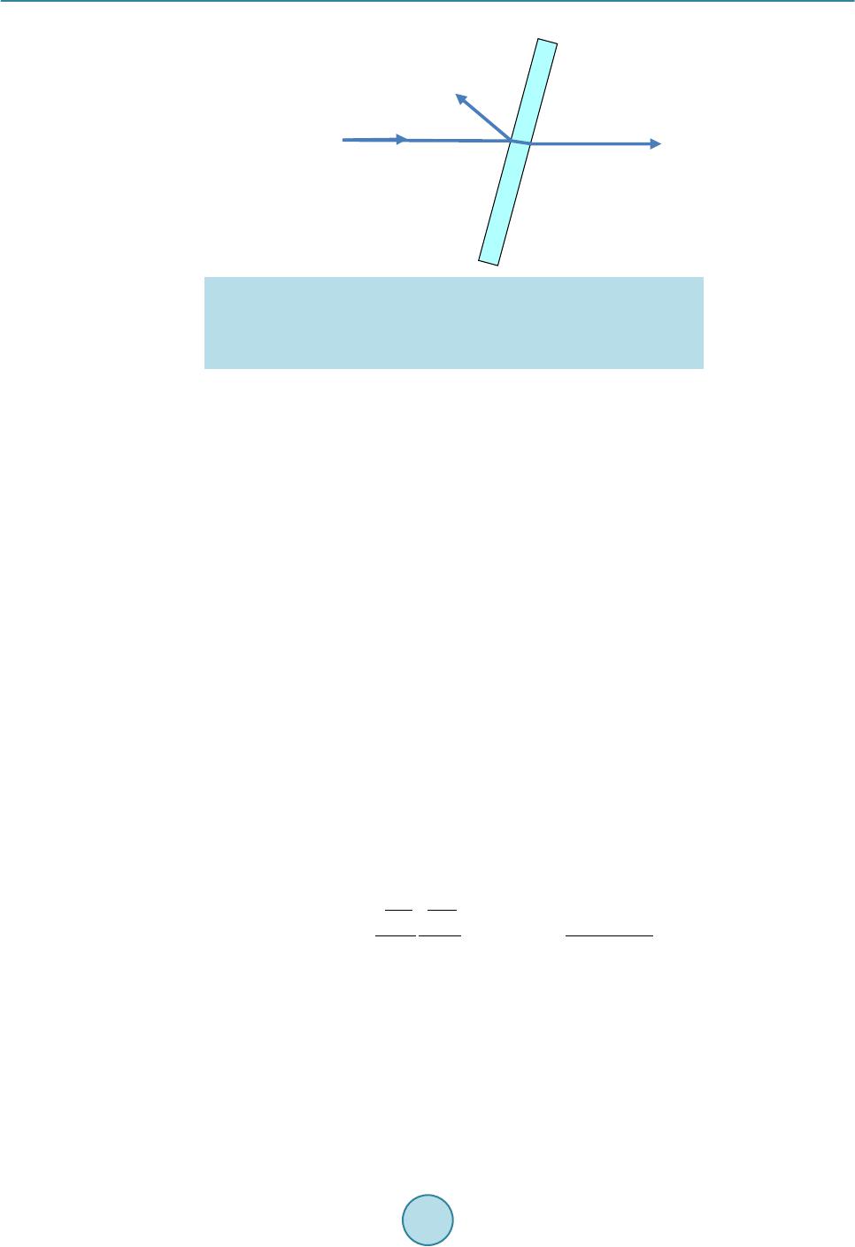

R. A. Hutchin
253
Figure 1. The simple reflection of an E&M wave off a dielectric interface has
been a huge challenge to a local theory of light. A local theory must identify a
deterministic cause for why a small fraction of the photons are reflected while
most transmit. The local theory for all angles and all refractive discontinuities
is presented below providing exact agreement with QM predictions.
1) When the photon comes to a refractive discontinuity, it can reflect or not.
2) To make that decision, it samples the local E & M wave pattern, which has two components—a transmitted
wave and a reflected wave.
3) Each of these two wave powers is multiplied by the vacuum field power at its particular wave vector at the
location o f the photon.
4) The photon then transitions to whichever path product has the larger magnitude.
This type of selection process would imply that the vacuum field may be involved in switching between can-
didate paths at a discontinuity.
While the detailed process of how the E & M and vacuum fields are sampled is not at all defined here (and
will have to wait for a field theory) , the probability calculation for th is process is straightforward. The probabil-
ity of selecting the weaker path is equal to the probability that the power of the weaker path times the pow er of
the vacuum field at that instant at that locatio n with the wave-number of the path is greater than the same type of
product for the stronger path. Since the local vacuum field amplitude for a particular wavevector is a Gaussian
random complex number (magnitude and phase), the magnitude-squared of the amplitude (which we are using
to decide which path t he photon will follow) will have an exponential distribution.
1 11
ProductE&M_Power VacuumPwr∗=
(13)
2 22
ProductE&M_Power VacuumPwr∗=
(14)
We will multiply each path power by the random exponential power appropriate to its wavevector, and then
have the photon go in the direction of the larger product. With this process, the probability of choosing the
weaker path 2 (P2) is given by the following double integral, where for conciseness we use Pwr1 and Pwr2 for
the transmitted and reflected path powers, and Vac1 and Vac2 for the vacuum field powers at each one’s wave-
vector.
12
112 2
2
2 12
00 12
eedd
vv
Vac Vac
PwrVacPwr Vac
vv
Pwr
PVac VacPwr Pwr
σσ
σσ
−−
∞<
== +
∫∫
(15)
We see that the resulting probability of the weaker path 2 being selected is exactly equal to its power com-
pared to the total path power, as we see experimentally and as is predicted by QM.
Thus we have shown is that it is possible to construct a random selection process between two possible pho-
tonic paths that matches current E & M predictions and experiments. That it uses the vacuum field with its h
factor is appealing because the randomness is completely independent at every reflection. There may, of course,
be other plausible options, but all of them will require the effect of a random number generator. Even QM says
that the choice is random without specifying the random process of selection. It is perhaps more difficult for QM
to find a plausible random number generator since the probability wave is distributed over a large area. Having
96%
4% Fused silica
plate
What deterministic process
makes a small fraction reflect?

R. A. Hutchin
254
the interaction confined to a point in space as the photon touches the discontinuity makes it very easy to use the
vacuum field—the univer se’s ubiqui tous rand om field.
This process of splitting the photonic flow at any discontinuity of the E & M wave is exactly what quantum
mechanics does. If the E & M wave (interpreted as a probab ility wave) splits at a discontinuity, then the proba-
bility of the photon going one way or the other splits proportionately. The key conclusion about this section and
its companion section 5 is that a local theory can distribute the flow of random photons identically to QM pre-
dictions even in the presence of discontinuous interfaces such as dielectric surfaces or polarizers. The rest of the
time, the photon is simply following the equivalent of the power flow of the E & M w ave—what QM interprets
as the probability flow. Thus the two look very close, except that the source of the randomness is clearly identi-
fied in the local theory as the vacuum field.
7. Malus’ Law—Polarized Photons through a Rotated Polarizer
In the case of polarized light passing through a polarizer rotated by angle θ (Figure 2), we will use the same
process as developed for partial reflection from a dielectric interface.
• When a photon arrives at the polarizing surface, it sees a refractive discontinuity with two E & M carrier
waves leaving that discontinuity—both of the proper frequency.
• Each path has a merit function equal to the power in its E & M wave times the magnitud e-squared of the in-
stantaneous vacuum field component at the wave-vector of each component.
• The phot on f ol l ows whichever path has t he larger product.
Just like with reflection from a dielectric surface , this process makes the probability of transmission or refle c-
tion for each photon proportionate to the relative power in each of the two E & M fields (transmitted and re-
flected). Since the transmitted carrier wave has a fraction of the power equal to cos(θ)2, that is the probability of
transmission. This is the essence of Malus’ Law and the result commonly reported by QM and experiment. This
simple process assures that the photon flux matches the E & M wave power at each beam splitter or polarizer.
Note: To get this probability calculation to match experiment, we had to assume that the photon did its selec-
tion independent of the polarization of the two candidate carrier waves (transmitted and reflected). Otherwise
whichever beam was closer to the incident polarization would have gotten a larger transmission—quite contrary
to experiment. This mathematical result suggests that the photonic singularity (which we have been calling the
photon) may not have a po larization associated with it at all b ut instead simply follows the E & M carrier wave
with whatever polarization it may have. Later experiments can test this hypothesis.
8. Local Waveforms that Satisfy Bell’s Test
The last challenge we consider for a local theory is Bell’s Theorem, which proves that two identical photons
cannot combine locally to match QM predictions for count correlations through polarizers. The typical experi-
mental layout and the verified QM prediction for count correlation are shown in Figur e 3. Experimentally,
scientists have worked quite hard to show that this barrier cannot be broken. Their experiments involve entan-
gled particles (today mostly entangled photons), and they compute a count statistic that Bell’s theorem says
cannot be reached by a local theory. Many such experiments have been done—all agreeing with quantum pre-
dictions.
In a previous paper [2] we relaxed the definition of “entangled photons” in a manner invisible to quantum
mechanics and found a local solution which bypassed Bell’s Theorem and did match QM predictions. By al-
lowing an entangled pair of photons to each has unobservable different properties, the QM predictions of count
Figure 2. The simple experiment shown above passes a fraction of the inci-
dent polarized photons through a polarizer rotated by angle θ. QM and expe-
riment say that fraction is cos(θ)2. A local theory must agree.
Pol 1Pol 2
Detecto r
Light
Source Lens
Dumps
Rotate by
angle θ
050100 150 200
0
0.2
0.4
0.6
0.8
1
POLARIZER ANGLE (DEG)
TRANSMISSION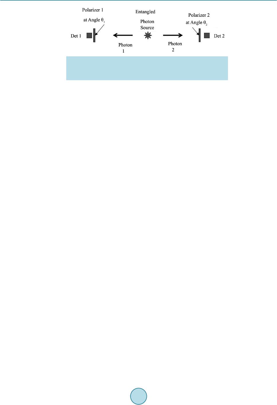

R. A. Hutchin
255
Figure 3. The Bell’s Theorem test of quantum mechanics uses a source of
entangled photons, where each photon goes to a different detector through
two different polarizers rotated at angles θ1 and θ2. The probability of simul-
taneous detection is proportional to cos(θ1 − θ2)2.
rate correlation with angle were matched, providing a local solution to Bell’s Test.
To get a local theory that matched QM predictions, we hypothesized a different excitation function with pola-
rizer angle for each of two types of photon, which together form an entangled pair. We called the excitation
functions simply P1(θ) and P2(θ), where θ = the angle between the photon polarization and the polarizer axis.
No one has ever found a way to measure the excitation function with angle of a single entangled photon, so
these local properties we hypothesized are “unmeasurable”—true hidden va ri ables.
We note that with this model, th e two photons are still tightly entangled in that if one has e xcitation function
P1(θ) then the other always has excitation function P2(θ) and vice versa. In simplest terms if one photon has a
detector response R1(θph − θpol) and the other has a detector response R2(θph − θ2pol), then if we average over
all internal photon angles θph, we get a correlation equal to the average of R1(θph − θ1pol) R2(θph − θ2pol) ove r θph,
which looks like a correlation function. The result mathematically must be cos(θ1pol − θ2pol)2. This is, of cou rse,
the QM and experimental result.
Once we allow the two entangled photons to be different in their response to a polarizer, then we quickly find
two responses with angle that together combine to match QM and experimental predictions. The two responses,
however, look strange to us. One response is a step function of period π, and the other is the positive part of
cos(2θ). As strange as they look, we note that no one has ever measured these two functions or even proposed a
technique for how to measure them. Since an entangled photon comes in a random and unknown polarization
state, there is no way to compare one transmission measurement with another, and thus no way to map out the
angular response of a single photon. We can only do correlations as in Bell tests.
We conclude that these two functions are true hidden variables, which have never been measured and may not
even be measureable. Even more, they constitute a mathematical proof that there are hidden variable formula-
tions of light that will match Bell tests by agreeing with QM predictions.
With this two-function modification to the definition of entangled photons, we have found a solution to their
count rates versus angle (plotted in Figure 4) that matched verified QM predictions. Here verification means
that the correlation between the two excitation functions equals the experimental result of cos(θ)2 − where θ =
the angle between the two polarizer axes.
Interpretation of the curves P1 and P2: Figur e 4 shows a purely mathematical result w hich says th at if two
entangle d ph otons produce the specified count probabilities with polarizer angle, then the count rates correlate to
match standard QM predictions between rotated polarizers. Now we must interpret these curves to connect to a
physical model.
The blue P2 curve is the easiest to interpret. It simply says that if the polarizer axis is within 45˚ of the photon
axis, then the Type 2 photon transmits through the polarizer; otherwise it ref lects .
The red P1 curve is more confusing at first. Yes the Type 1 photon transmits or reflects in the same quadrants
as the Type 2 photon, but what does it mean to have more or less than one count for a single photon? The overall
count average is unity over each transmissive quadrant, but what do the variations mean?
We find a clue in a previous paper [10], which showed that all photonic interactions (excitation and stimu-
lated emission) have the same universal cross-section given by Co = λ2/2π, when averaged over all polarizations
and directions. (This paper was based on Einstein’s 1917 paper on stimulated emission [7].) Given a theor y with
two types of photons, we suggest that what can vary is the photonic cross-section. A value of 1 would indicate a
cross-section of Co.
If this interpretation is correct, then we have a plausible interpretation of the variable count rates in Figure 4,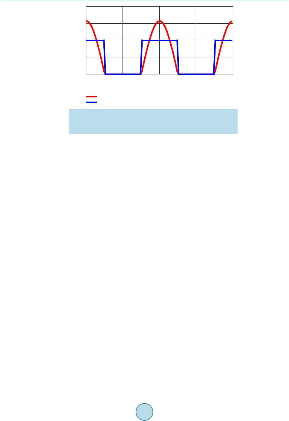

R. A. Hutchin
256
Figure 4. Plot of two photon response functions, P1 and P2, which cross-
correlate to give the experimental cos(θ)2 polarization correlation predicted
by QM and verified experimentally. The horizontal axis is the difference be-
tween the angle of the photon’s polarization and the angle of the polarizer.
and we also have immediate physical consequences which can be verified in Bell Test experiments.
9. High QE Test of a Local Theory vs QM
In presenting any local theory as a competitor to the QM theory of light, it is important to identify potential ex-
perimental situations which might distinguish between the two. After all, nature will be one way or the other.
Since classical E & M theory already provides the same predictions as QM theory for many phenomena, we
must go to some effort to find an experiment that will separate the local from the quantu m theories. No t surpri-
singly, we have found that the local theory agrees perfectly with QM at low quantum efficiency, but we predict
deviations from the QM predictions for count correlations with entangled photons at high quantum efficiency.
That theory is presented below. It is likely that the data to test these pr edictions already exists, but has not been
processed in the way proposed here.
To make this analysis precise, we need an equation for the probability of detection that depends on the inte-
raction cross-section. We make this model quite simple. We assume we have a detector material of thickness d
which has a uniform random density ndet of detection sites/unit volume. Typically a detection site would be an
atom or molecule with an electron that can be excited into a conduction band. We assume that these detection
sites are distributed randomly throughout the detector material.
Using this simple model, we compute the probability of detection as follows: Each photon will follow a line
path through the detector material, creating an interaction volume of its cross-section Cph times the thickness d.
The photon’s probability of being detec ted will then be equal to the probability that th is path of volu me V = Cphd
includes a detection site.
Using the familiar Pois son statistics for a randomly distributed se t of points, we compute that the probab ility
of there being no detection is equal to the probability that there is no detection site in the interaction volume =
exp(−ndetCphd). One minus that probability would then be the probability of being detected as given in Equation
(16). The probability of detection is, of course, simply called the quantum efficiency of the detector, which va-
ries with the cross-section of the photon.
( )
( )
1e
detph
nCd
det ph
PC
−
= −
(16)
Using the definition of quantum efficiency to be the mean detection probability over all photon angles and
configurations, we should get the measured QE when Cph = Co, its mean value as shown in Equation (17).
( )
1e
det o
n Cd
QE
−
= −
( 17)
Now we can solve for the quantity ndetd in Equation (16) and substitute the result into Equation (15) to get
090180 270360
0
0.5
1
1.5
2
P1
P2
ANGLE BETWEEN PHOTON AND POLARIZER (DEG)
COUNT PROBABILITY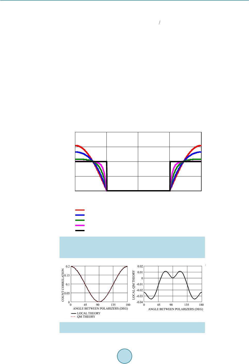

R. A. Hutchin
257
Equation (17) that uses only known quantities: the mean detector QE (measured by the manufacturer) and the
photon interaction level divided by Co, plotted in Figure 5.
( ) ( )
( )
11
ph o
CC
det ph
P CQE=−−
We apply this formula as shown in Figure 5 to compute the relative probability of detection for type 1 and
Type 2 photons versus the angle between their polarization axis and the polarizer. That relative probability is
plotted for 5 different level of quantum efficiency, QE, in Figure 5. In a test of Bell’s Theorem, the prob ability
of detecting a Type 1 photon will then vary within a quadrant, while the probability of detection for a Type 2
photon will be consta nt in each quadrant.
Using this model for the local interaction theory, we can convolve the type 1 and type 2 curves in Figure 5, to
compute the count correlation for each level of quantum efficiency, QE. The deviation from QM predictions for
the above local theory is quite s mall when the detector QE < 0.2 and quite substantial when the QE = 0 .99. The
comparison of local to QM predictions at QE = 0.2 is shown in Figure 6. W h en t he QE of a detector is this low,
this effect is almost invisible on a plot, but it can be seen numerically if the stability and count statistics of the
experiment are sufficient. When the QE is 0.99, the deviation is large and easily seen on a plot or with analysis.
Figure 7 shows this case.
Local versus QM Metric: We recommend the following metric as a test for locality, using three popular
measurement angles (22.5˚. 67.5˚ and 90˚). The ratio between the local theory and QM predictions is plotted
versus Quantum Efficiency in Figure 8, showing how sensitive it is to QE getting close to unity. It is 0.707 for
Figure 5. Here the interaction cross-section is plotted versus the angle be-
tween the Type 1 photon and the polarizer as a function of the quantum effi-
ciency (QE) of the detector. Since the magnitude and shape change with QE,
the local theory predicts deviations from QM predictions at high QE.
Figure 6. At detector QE = 0.20 the deviation between QM and local predic-
tions is −0.0035 to +0.0011.
045 90 135 180
0
0.5
1
1.5
2
QE = 0.05
QE = 0.50
QE = 0.90
QE = 0.99
QE = 1.00
ANGLE BETWEEN PHOTON AND POLARIZER (DEG)
TYPE 1 CROSS-SECTION/Co

R. A. Hutchin
258
Figure 7. At QE = 0.50,0.90, 0.99 and 1.00 the deviation between QM and local predictions is a maximum at
polarizer angles 22.5˚ and 67.5˚, two angles frequently in Bell tests.
Figure 8. The Local vs QM metric is plotted here versus quantum efficiency (QE). The QE here does not in-
clude transmission loss factors along the path—just the detector. This metric is proportional to the transmis-
sion, but the fractional change between the local and QM predictions is unchanged.
04590135 180
0
0.1
0.2
0.3
0.4
LOCAL THEORY
QM THEORY
ANGLE BETWEEN POLARIZERS (DEG)
COUNT CORRELATION
04590 135 180
0
0.2
0.4
0.6
0.8
LOCAL THEORY
QM THEORY
ANGLE BETWEEN POLARIZERS (DEG)
COUNT CORRELATION
045 90135 180
0
0.2
0.4
0.6
0.8
LOCAL THEORY
QM THEORY
ANGLE BETWEEN POLARIZERS (DEG)
CO UNT C OR R ELA TI ON
Q
04590135 180
0
0.2
0.4
0.6
0.8
LOCAL THEORY
QM THEORY
ANGLE BETWEEN POLARIZERS (DEG)
COUNT CORRELATION
QE = 0.50QE = 0.90
QE = 0.99QE = 1.00
LocalMetric Sig 22.5deg⋅() Sig 67.5 deg⋅( )−
Sig 22.5 de g⋅() Sig 67.5deg⋅( )+2Sig 90 deg⋅( )⋅ −
00.1 0.2 0.3 0.4 0.5 0.6 0.7 0.8 0.91
0
0.1
0.2
0.3
0.4
0.5
0.6
0.7
0.8
LOCAL THEORY
QM THEORY
QUANTUM EFFICIENCY
LOCAL METRIC

R. A. Hutchin
259
all conditions with QM models and less than that fo r th e local theor y of ligh t.
10. Summary
We have explored a local theory of light by addressing fo ur historically difficult qu es tions:
How can a local theory of light:
1) Explain spontaneous emission of light?
2) Explain partial reflection at a dielectric inte rface?
3) Explain partial reflection from a polarizer (Malus’ Law)?
4) Match QM results for count correlations of entangled photons?
In the first three questions we found the key in the vacuum E & M field, which provided the source for spon-
taneous emission as well as the random number generator required for each photon to decide to reflect or not at
a dielectric interf ace or a polarizer. QM is all about probabilistic ou tcomes, which require so mewhere in nature a
suitable random number generator. Our exploration of Questions 1, 2 and 3 suggest that the vacuum field may
be central to that process—the universe’s only known ubiquitous random number generator.
Question 4 (Bell’s Test) was answered using a previous paper [2] on a local theory that agreed with quantum
mechanics on Bell tests with entangled photons. However, in this paper we dived much more deeply to explore
the physical consequences and interpretations of the local solution that emerged. The result of that deeper inves-
tigation was a correlation test for a local theory versus a QM theory of light which took advantage of the higher
QE detectors available today for Bell testing.
11. Conclusion
The huge simplification in physics that would accompany the transition from a QM theory to a local theory
compelled us (as it has others) to explore a local theory of light. Once Bell’s Theorem had been bypassed ma-
thematically [2], it seemed appropriate to explore the p ath to a local theory more intensely. Here we have shown
possible local solutions to four h istorical barriers to a local field: spontaneou s emission, partial r eflection at a di-
electric interface, partial reflection of polarized light from a polarizer, and Bell tests. An experiment which can
distinguish between a local and QM model of light has been suggested. If such an experiment shows deviations
from QM predictions, then the door will be opened to a local theory of light. Such experimental data may al-
ready exist in previous data sets using high QE detectors.
References
[1] Hutchin, R.A. (2015) A New Physical Model for the Vacuum Field Based on Einstein’s Stimulated Emission Theory.
Optics and Photonics Journal, 5, 109-112. http://dx.doi.org/10.4236/opj.2015.54009
[2] Hutchin, R.A. (2015) A Local Theory of Entangled Photons That Matches QM Predictions. Optics and Photonics
Journal, 4, 304-308. http://dx.doi.org/10.4236/opj.2014.410030
[3] Barrow, J.D. and Tipler, F.J. (1986) The Anthropic Cosmological Principle. Oxford University Press, Oxford.
[4] Faria, A.J., Franca, H.M., Gomes, G.G., et al. (2006) The Va cuum Elect r omagneti c Fields and the Schrödinger Picture.
[5] Casimir, H.B.G. (1948) On the Attraction between Two Perfectly Conducting Plates. Proc. Kon. Nederland. Akad.
Wetensch. B51, 793-795.
[6] Bordag, M., Mohideen, U. and Mostepanenko, V.M. (2001) New Developments in the Casimir Effect. Physics Reports,
353, 1-205. http://dx.doi.org/10.1016/S0370-1573(01)00015-1
[7] Einstein, A. (1917) Zur Quantentheorie der Strahlung (On the Quantum Theory of Radiation). Physika Zeitschrift, 18,
121-128.
[8] Clauser, J.F. (1974) Experimental Distinction between the Quantum and Classical Field-Theoretic Predictions for the
Photoelectric Effect. Physical Review D, 9, 853. http://dx.doi.org/10.1103/PhysRevD.9.853
[9] Adler, R., Basin, M. and Schiffer, M. (1965) Introduction to General Relativity. McGraw-Hill, Boston.
[10] Hutchin, R.A. (2015) Universal Cross-Section of Photonic Interaction. Optics and Photonics Journal, 5, 109-112.
http://dx.doi.org/10.4236/opj.2015.54009