Applied Mathematics, 2011, 2, 830-835
doi:10.4236/am.2011.27111 Published Online July 2011 (http://www.SciRP.org/journal/am)
Bayes Shrinkage Minimax Estimation in Inverse
Gaussian Distribution
Gyan Prakash
Department of Community Medicine, Sarojini Naidu Medical College, Agra, India
Received November 19, 2010; revised May 14, 2011; accepted May 17, 2011
Abstract
In present paper, the properties of the Bayes Shrinkage estimator is studied for the measure of dispersion of
an inverse Gaussian model under the Minimax estimation criteria.
Keywords: Bayes estimator, Bayes Shrinkage estimator, Uniformly Minimum Variance Unbiased Estimator
(UMVUE), LINEX loss function (LLF) and Minimax Estimator
1. Introduction
The Inverse Gaussian distribution plays an important role
in Reliability theory and Life testing problems. It has
useful applications in a wide variety of fields such as
Biology, Economics, and Medicine. It is used as an im-
portant mathematical model for the analysis of positively
skewed data. The review article by Folks & Chhikara
[1,2] and Seshadri [3] have proposed many interesting
properties and applications of this distribution.
Let 12 be a random sample of size
drawn from the inverse Gaussian distribution
,,,,
n
x x x,n


μθIG , :
having probability density function
 
2
32
;, exp ;
22
0, ,0
θ xμ
θ
f x μθ
π xμx
x θ .








(1)
Here,
μ
stands for the mean and for the inverse
measure of dispersion. The maximum likelihood esti-
mates of
θ
μ
and θ are given as:
1
1
ˆi
n
i
μ x x
n

 andˆ
,
n
θ
v

where
1
11
.
i
n
i
v
xx






The unbiased estimates of
μ
and θ are respect-
tively
x
and

13
u
θn
v


. Also, ~
x


IG, , μnθ

1n
θ v ~ χ 
2 with and being stochastically inde-
pendent ( [1,4,5,]).
Schuster [6] showed that

2
2
1
ni
ii
x
μ
θ
x μ

is distributed as chi–square distribution
with degrees of freedom. If we assume that n0 μ
μ

is known, the uniformly minimum variance unbiased
(UMVU) estimator for measure of dispersion, 1 θ

is

2
0
2
10
1ni
ii
xμ
U
nxμ


 (2)
and follows a chi-square distribution with
degrees of freedom.
Un θn
The choice of the loss function may be crucial. It has
always been recognized that the most commonly used
loss function, squared error loss function (SELF) is in
appropriate in many situations. If the SELF is taken as a
measure of inaccuracy then the resulting risk is often too
sensitive to the assumptions about the behavior of the tail
of the probability distribution. In addition, in some esti-
mation problems overestimation is more serious than the
underestimation, or vice-versa [7]. To deal with such
cases, a useful and flexible class of asymmetric loss
function (LINEX loss function (LLF)) was introduced by
Varian [8]. The reparameterized version of LLF ([9]) for
any parameter is given as
θ


ˆ
1; 0 and .
a
Le a a θθθ

  (3)
The sign and magnitude of ‘a’ represents the direction
and degree of asymmetry respectively. The positive
(negative) value of ‘a’ is used when overestimation is
v
x

G. PRAKASH 831
more (less) serious than underestimation.

L

is ap-
proximately square error and almost symmetric if a
near to zero.
Thompson [10] suggested a procedure, which makes
use of a prior information of the parameter in form of a
guessed value by shrinking the usual unbiased estimator
towards the guess value of the parameter with the help of
a shrinkage factor . The experimenter ac-
cording to his belief in the guess value specifies the val-
ues of shrinkage factor. The shrinkage estimator for the
measure of dispersion of when a guess
value of say is available, is given by

0k k
1
θIG
0,

1

.

, μθ
,θ θ

1
0
ˆ1 ; 01
Sk θkθk

  (4)
Some shrinkage estimators for measure of dispersion
have been obtained by Pandey & Malik [11] and
have studied their properties under SELF–criterion.
Prakash and Singh [12] have studied the properties of
different shrinkage testimators for under the LINEX
loss function. Palmer [13] and Banerjee & Bhattacharya
[14] have discussed the Bayesian inference about the
parameters of the inverse Gaussian distribution.
1
θ
1
θ
The present article proposed Bayes Shrinkage estima-
tor based on the Minimax criteria for the measure of dis-
persion. A Bayes estimator for the measure of dispersion
under the vague prior has been obtained in the Sec-
tion 2. Under the Minimax criteria the Bayes Minimax
estimator has been obtained in the Section 3. A Shrink-
age estimator construct by utilizing the Bayes Minimax
estimator in the Section 4. Further, a numerical study has
been presented in Section 5 and draws a conclusion about
the Bayes Shrinkage Minimax estimator in Section 6.
1
θ
2. Bayes Estimator for Measure of
Dispersion
We are not going into debate or to justify the questions
of the proper choice of the prior distribution. We con-
sider a vague prior for the parameter

which is an
increasing function of the parameter

and is given as
(); 0.
d
gθθd
Therefore, the posterior density of parameter

is
defined as
 
 
22
;
π=; ;
;d
nn U
LUθg θ
θLUθθe
L Uθ g θθ





After simplifying, the posterior density of parameter

is obtained as

1 1
222
π1
22
n d nn θ
d U
nnU
θΓ d θe
 



 

 . (5)
The Bayes estimator for the measure of dispersion
1
θ

ity
under the LLF is obtained by simplifying the equal-



ˆ.
a θθ a
pp
EθeeEθ
Here, the suffix indicates that the expectation is
taken under poensity. After simplification the
Bayes estimator for
p
sterior d
θ1

under the LLF is
2
ˆ; 1exp.
224
n a
θU a n d 



 



(6)
3. The Minimax Bayes Estimator
The basic principle of this approach is to minimize the
n a theorem,
n be stated as
loss. The derivation depends primarily o
given by Hodge & Lehmann [15] and ca
follows.
Let


:
θ
ωFθ

 be a family of distribution func-
tions and C be a class of estimators of the parameter

. Suppose that * cC

is a Bayes estimator against a
prior distribution


θ on the parameter space g

.
Then the Bayes estimator *
c is said to be the Minimax
e timator if the riction of the estimator *
c is in-
dependent on
ssk fun

.
Here, the risk of the Bayes estimator

given in (6)
for the parameter 1
θ

with respect to LLF is dened as fi






11Δ
ˆ
() a
RθfU eˆ

Δ1d ; Δ
U
a Uθθ θ 
(7)
Since, nU

is distributed as a Chi-square with n
degrees of freedom. Then by making a transformn atio
2
nU
z

, the distribzution of is obtained as

11
n
z
n

 2; 0
2
fz ezz



 (8)
Using equation (8) in the expression we have

ˆ
Rθ



2
1
2
0
Γ
2
nn
2
12
ˆ1d
2
ˆ
111.
a nz
za
n
n
a
a
Rθezeez az
a
Rθea
n



















 (9)

 



The Equation (9) represents the risk of the Bayes esti-
mator of the measure of dispersion, which is independent
with the parameter

. Hence, the Bayes estimator

is
th
y
rent
e Minimax estimator under the LLF loss criterion.
The following statistical problem (Minimax Estima-
tion) is equivalent to some two person zero sum game
between the Statistician (Player–II) and Nature (Plaer–
I). Here the pure strategies of Nature are the diffe

G. PRAKASH 832
values of

in the interval

0, and the mixed
strategies of Nature are the prior densities of

in the
interval

0,. The pure strategies of Statistician are all
possible decision functions in the interval

0,.
The expected value of the loss function is the risk
function and it is the gain of the Player–I. Furher, the
Bayes risefined as
ˆˆ
t
k is d
 
, θ
Rηθ ERθ
Here, the expectation has been taken under the prior
density of parameter

. If the loss function is continu-
ous in both the estim and thearameterator ˆ
θ p

, and
convex in for e of
ˆ
θeachvalu

then therist
m
e ex
easures * η and ˆ * θ for all

and ˆ θ so that, the
following relation holds:
 
ˆˆˆ
,,,
****
RηθRηθ Rηθ
The number

ˆ
,
**
Rηθ is known as th value of the
game, and *
η and ˆ * θ a
e
re the corresponding optimum
strategies of tand II. In statisticas is
the least fansity of
h
vora
e Player I
ble prior de
l term*
η

and the estimtor
for
a
ˆ* is the Miniator. In fact, the value of the
game is the loss of the Player–II. Hence, the optimum
strategy of Player–II and the value of game are given
present case as
Optimum
Strategy
Corresponding
Loss Value of Game
θmax estim
ˆ
θU

 LLF

2
2
1
n
aa
ea
n






1 1 
4. The Shrinkage Bayes Minimax Estimator
Now, we construct a Shrinkage Bayes Minimax estima-
tor as


1
1. θUθ 

 (10)
0
The risk of the Shrinkage Bayes Minimax estimator
θ under the LLF is obtain by using Equation (8) as




 

Δ Δ 1d
24
11 1
a
RθfU eaU
n d
aδ 




 

(11)
where
U
exp 1expan Rθ aδa 

 


11
Δ θθθ

 and
The comparison of the considnkage Bayes
Minimax estimator
1
0.
δθθ


ered Shri
θ is performs with the help of a
minimum class of estimator based on the UMVU esti-
Here, the consideredof estimar based on
U
mator. class to
MVU estimator is
; .TlUlR

 (12)
The risk of the estimator T under the LINEX loss is
given by
 
1.l
2
2
11
n
aal
RT ea


n



, which minimizes is given by


The constantl

RT
2
1exp .
22
na
l an











(13)
ng the
with the risk under the LLF is given as
Thus, the improved estimators amo class T is
TlU

 (14)

2
1exp1.
n a
RT a

 
22n


(15)



of


Remark: It observed that the value

rame
um
is lies be-
tween zero and one for the selected patric set of
values which are considered later for the ne
ings. Therefore,
rical find-

is considered as the shrinkage factor.
max estimator
5. A Numerical Study
The relative efficiencies for the Shrinkage Bayes Mini-
θ relative to the improved estimator
T

is defined as



, .
RT
RE θTRθ

The relative

efficiencies are the functions of
and For the selected set of val
,n
ues
,a
of δ
n
.d
15,205,10, 5;

025,050; a. .


,01,150,02,05;.
025(..025)175. δ
and 025d.,050.

the relative efficiency
e re-ha
sen
ve been calculated. The numerical findings arp
ted hernly for 05n
e o

and 15n in the Tables
It is obge Bayes Minimax esti-
mator
1 and 2 respectively.
served that the Shrinka
θ is performs better then the improved estimator
T

for the all selected parametr
025175.δ.
ic set of values for

. Furthmple size increases the
re
er, as san
lative efficiency decreases for all considered paramet-
ric set values and attains maximum efficiency at the
1δ
of
point

. Further, it is also observed that the relative
eases as d increases when δ lie be-
tween 050 150.δ.
efficiency incr

. It is seen also that, as ‘a’ in-
crease relative efficiency first increases for 075δ.

and thecrease for the other values of δ.
6. Con
In present paper we obtained the Shrin ag
n de
clusions
ke estimator

G. PRAKASH 833
ax estimation criteria for the measure
of dispersion of the inverse Gaussian distribution. We ob-
based on the Minimserved that on the basis of the relative efficiency, the pro-
posed Shrinkage Bayes Minimax estimator θ performs
θ Table 1. Relative efficiency for the estimator with respect toes
.
0.25
* T under LLF for n = 5 and different valuof a, d and
δ
0.5 1 1.5 2
a δd
0.25 1 1 1. 1..1782.15921127 1.06330161
0.50 1.6600 1.7066 1.7695 1.8010 1.8110
0.75 2.2234 2.4028 2.7503 3.0766 3.3768
1.00 2.5931 2.8804 3.5000 4.1796 4.9192
1.25 2.4673 2.6799 3.0899 3.4717 3.8190
1.50 1.9834 2.0465 2.1276 2.1635 2.1698
–0.05
–0.25
0.25
0.05
1.75 1.4748 1.4525 1.3928 1.3276 1.2655
0.25 1.1923 1.1737 1.1282 1.0797 1.0332
0.50 1.6869 1.7333 1.7953 1.8258 1.8348
0.75 2.2582 2.4388 2.7880 3.1147 3.4144
1.00 2.5904 2.8733 3.4829 4.1511 4.8778
1.25 2.3821 2.5787 2.9575 3.3106 3.6324
1.50 1.8466 1.9002 1.9698 2.0017 2.0086
1.75 1.3356 1.3150 1.2628 1.2069 1.1534
0.25 1.2177 1.2002 1.1567 1.1102 1.0655
0.50 1.7353 1.7815 1.8422 1.8710 1.8782
0.75 2.3158 2.4996 2.8530 3.1816 3.4808
1.00 2.5583 2.8327 3.4233 4.0697 4.7719
1.25 2.1896 2.3589 2.6853 2.9902 3.2694
1.50 1.5808 1.6218 1.6772 1.7054 1.7149
1.75 1.0847 1.0695 1.0323 0.9924 0.9538
0.25 1.2292 1.2121 1.1698 1.1244 1.0806
0.50 1.7570 1.8032 1.8634 1.8914 1.8980
0.75 2.3391 2.5247 2.8807 3.2106 3.5099
1.00 2.5301 2.8004 3.3819 4.0179 4.7085
1.25 2.0860 2.2438 2.5482 2.8330 3.0944
1.50 1.4546 1.4915 1.5427 1.5704 1.5816
1.75 0.9732 0.9609 0.9305 0.8975 0.8651

G. PRAKASH 834
Table 2. Relative efficiencthe estimator y for θ with respect under LLd δ.
0.25 .5
to * T F for n = 15 and different values of a, d an
a δd 01 1.5 2
0.25 1 1 1.0109 0.9659 0.9182 .0624 .0484
0.50 1.2457 1.2660 1.2949 1.3099 1.3134
0.75 1.4014 1.4590 1.5717 1.6804 1.7841
1.00 1.4912 1.5691 1.7308 1.9004 2.0780
1.25 1.4755 1.5432 1.6762 1.8048 1.9277
1.50 1.3723 1.4048 1.4538 1.4835 1.4967
–0.05
–0.25
0.25
0.05
1.75 1.2137 1.2068 1.1766 1.1323 1.0812
0.25 1.0718 1.0584 1.0219 0.9777 0.9308
0.50 1.2612 1.2825 1.3130 1.3291 1.3335
0.75 1.4171 1.4759 1.5911 1.7021 1.8080
1.00 1.4875 1.5658 1.7285 1.8991 2.0777
1.25 1.4557 1.5196 1.6447 1.7654 1.8807
1.50 1.3262 1.3532 1.3930 1.4159 1.4246
1.75 1.1480 1.1375 1.1038 1.0595 1.0107
0.25 1.0895 1.0773 1.0428 1.0004 0.9548
0.50 1.2898 1.3132 1.3470 1.3656 1.3718
0.75 1.4427 1.5043 1.6247 1.7407 1.8513
1.00 1.4875 1.5645 1.7244 1.8920 2.0674
1.25 1.4012 1.4580 1.5689 1.6757 1.7775
1.50 1.2222 1.2406 1.2665 1.2796 1.2822
1.75 1.0133 0.9990 0.9631 0.9215 0.8782
0.25 1.0979 1.0862 1.0527 1.0112 0.9664
0.50 1.3031 1.3274 1.3630 1.3829 1.3900
0.75 1.4528 1.5158 1.6390 1.7577 1.8708
1.00 1.4803 1.5569 1.7158 1.8825 2.0568
1.25 1.3675 1.4210 1.5257 1.6263 1.7221
1.50 1.1660 1.1812 1.2021 1.2119 1.2127
1.75 0.9462 0.9313 0.8959 0.8566 0.8164
etter than an improved estiator in a wide of
d R. S. Chhikara, “The Inverse Gaussian
Distribution Its Statistiation—,”
Journal of the Royal Statistical Society, Vol. 40, No. 3,
b
w
me rangδ
hich is defined here as the ratio between the true value
and guess (prior point) value of the unknown parameter
under the LLF. Thus, we suggest using the Minimax es-
timator under LLF for estimating the measure of disper-
sion under the Shrinkage setup.
7. References
[1] J. L. Folks an
andcal ApplicA Review
1978, pp. 263-289.
[2] J. L. Folks and R. S. Chhikara, “The Inverse Gaussian
Distribution,” Marcel Dekker, New York, 1989.
[3] V. Seshadri, “The Inverse Gaussian Distribution,” Statis-
tical Theory and Applications, Springer–Verlag, New
York, 1998.
[4] M. C. K. Tweedie, “Statistical Properties of Inverse Gau-
ssian Distribution–I,” The Annals of Mathematical Statis-

G. PRAKASH 835
No. 2, 1957, pp. 362-377. tics, Vol. 28,
doi:10.1214/aoms/1177706964
[5] M. C. K. Tweedie, “Statistical Properties of Inverse
Gaussian Distribution–II,” The Annals
Statistics, Vol. 28, No. 2, 1957, p
of Mathematical
p. 696-705.
doi:10.1214/aoms/1177706881
[6] J. J. Schuster, “On the Inverse Gaussian Distribution,”
Journal of American Statistical Association, V
324, 1968, pp. 1514-1516.
ol. 63, No.
.2307/2285899doi:10
Applied
etrics and Statistics, Amsterdam
ommunication in Sta-
[7] A. Parsian and S. N. U. A. Kirmani, “Estimation under
LINEX Loss Function,” In: A. Ullah, A. T. K. Wan, A.
Chaturvedi and M. Dekker, Eds., Handbook of
Econometrics and Statistical Inference, CRC Press, Boca
Raton, 2002, pp. 53-76.
[8] H. R. Varian, “A Bayesian Approach to Real Estate As-
sessment,” In: S. E. Feinberge and A. Zellner, Eds., Stud-
ies in Bayesian Econom
North Holland, 1975, pp. 195-208.
[9] D. C. Singh, G. Prakash and P. Singh, “Shrinkage Testi-
mators for the Shape Parameter of Pareto Distribution
Using the Linex Loss Function,” C
tistics: Theory and Methods, Vol. 36, No. 4, 2007, pp.
741-753. doi:10.1080/03610920601033694
[10] J. R. Thompson, “Some Shrinkage Techniques for Esti-
mating the Mean,” Journal of the American Statistical
Association, Vol. 63, No. 321, 1968, pp. 113-122.
doi:10.2307/2283832
[11] B. N. Pandey and H. J. Malik, “Some Improved E
tors for a Measure of
stima-
Dispersion of an Inverse Gaussian
Distribution,” Communications in Statistics: Theory and
Methods, Vol. 17, 1988, pp. 3935-3949.
doi:10.1080/03610928808829847
[12] G. Prakash and D. C. Singh, “Shrinkage
the Inverse Dispersion of the Inve
Testimators for
rse Gaussian Distribu-
,” Ph.D.
-
tion under the Linex Loss Function,” Austrian Journal of
Statistics, Vol. 35, No. 4, 2006, pp. 463-470.
[13] T. Palmer, “Certain Non-Classical Inference Procedures
Applied to the Inverse Gaussian Distribution
Dissertation, Oklahoma State University, Stillwater, 1973.
[14] A. K. Banerjee and G. K.Bhattacharya, “Bayesian Results
for the Inverse Gaussian Distribution with an Applica
tion,” Technometrics, Vol. 21, No. 2, 1979, pp. 247-251.
doi:10.2307/1268523
[15] J. I. Hodge and E. L. Lehmann, “Some Problems in
Minimax Estimation,” Annals of Mathematical Statistics,
Vol. 21, No. 2, 1950, pp. 182-197.
doi:10.1214/aoms/1177729838
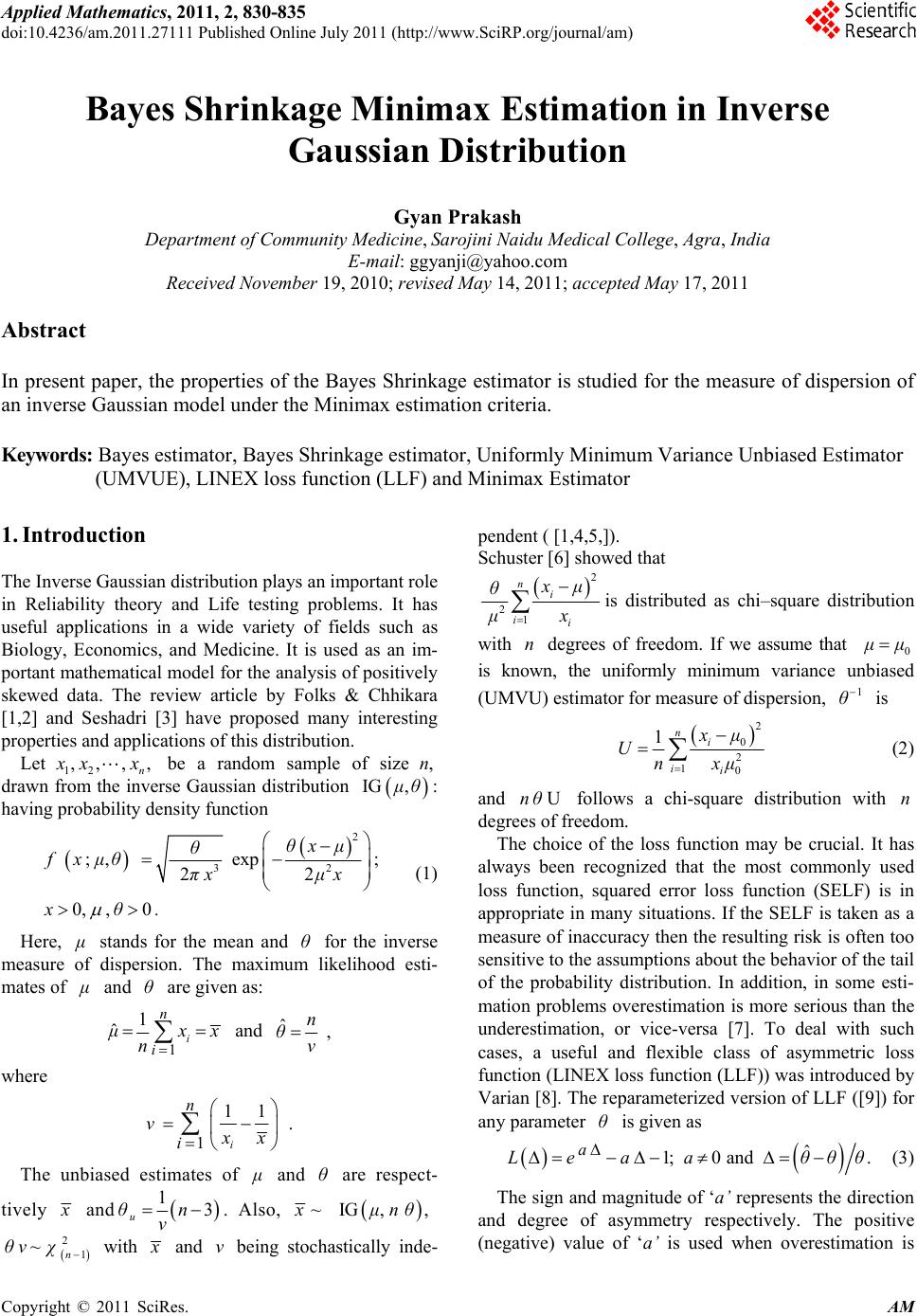