 American Journal of Computational Mathematics, 2011, 1, 55-62 doi:10.4236/ajcm.2011.12006 Published Online June 2011 (http://www.scirp.org/journal/ajcm) Copyright © 2011 SciRes. AJCM 55 Numerical Solution of Obstacle Problems by B-Spline Functions Ghasem Barid Loghmani1, Farshad Mahdifar2, Seyed Rouhollah Alavizadeh1 1Department of Mat hem at i cs, Yazd University, Yazd, Iran 2Department of Mat hem at i cs, Payame Noor University, Tehran, Iran E-mail: loghmani@yazduni.ac.ir, farshad.mehdifar@pnu.ac.ir Received February 19 , 20 11; revised April 6, 2011; accepted April 15, 2011 Abstract In this study, we use B-spline functions to solve the linear and nonlinear special systems of differential equations associated with the category of obstacle, unilateral, and contact problems. The problem can easily convert to an optimal control problem. Then a convergent approximate solution is constructed such that the exact boundary conditions are satisfied. The numerical examples and computational results illustrate and guarantee a higher accuracy for this technique. Keywords: Least Square Method, Uniform B-Splines, Boundary Value Problems, Obstacle Problems 1. Introduction Variational inequality theory has become an effective and powerful tool for studying obstacle and unilateral problems arising in mathematical and engineering sci- ences. This theory has developed into an interesting branch of applicable mathematics, which contains a wealth of new ideas for inspiration and motivation to do research. It has been shown by Kikuchi and Oden [1] that the problem of equilibrium of elastic bodies in contact with a right foundation can be studied in the framework of variational inequality theory. Various numerical me- thods are being developed and applied to find the nume- rical solutions of the obstacle problems including finite difference techniques and spline based methods. In principle, these methods cannot be applied directly to solve the obstacle problems. However, if the obstacle function is known, one can characterize the obstacle problem by a sequence of boundary value problems without constraints via the variational inequality and a penalty function. The computational advantage of this approach is its simple applicability for solving diffe- rential equations. Such type of penalty function methods have been used quite effectively by Noor and Tirmizi [2], as a basis for obtaining numerical solutions for some obstacle problems. The aim of this paper is to consider the use of quadratic B-spline functions and least square method to develop a numerical method for obtaining smooth appro- ximations for the solution and its derivatives of the general form of a system of second order boundary value problem of the type. 11 22 33 (, (), ()),= ()=(, (), ()), (, (), ()),= 2 3 4 tut utaata utgtut utata tut utatab (1) 1 ()=ua and 2 ()=ub , (2) and the continuity conditions of and at 2 a and 3. Here, (i), are given continuous functions, and the parameters 1 uu =1,a2 1 :[, ] iii gab RR 2, 3 and 2 are real finite constants. Linear form of such type of systems arise in the study of one dimensional obstacle, unilateral, moving and free boundary value problems, [1,3-10] and the references therein. In general, it is not possible to obtain the analytic form of the solution of (1)-(2) for arbitary choices of i(, , ) tuu , ( ), so we resort to some numerical methods for ob- taining an approx imate solution of (1)-(2). =1i, 2, 3 In 1981, Villaggio [11] used the classical Rayleigh- Ritz method for solving a special form of (1), namely, 3 0,0 and 44 ()= 3 () 1,44 tt ut ut t (3) (0) =0u and ()=0u , (4) and the continuity conditions of and u at u4 and  56 G.B. Loghmani ET AL. 34 . Later, Noor and Khalifa [12] have solved problem (3)-(4) using collocation method with cubic splines as basis functions. Similar conclusions were pointed out by Noor and Tirmizi [2], Al-Said [13] and Al-Said et al. [14], where second and fourth order finite difference and spline methods were used to solve a special linear form of problem (1), namely, 23 23 (), and ()= () ()(), ft ataatb ut gtutft r ata (5) 1 ()=ua and 2 ()=ub . (6) where, the functions () t and () t are continuous on [a, ] and [, 3], respectively and the continuity conditions of and at 2 and 3 is assumed, and is a real finite constants parameter. On the other hand, Al-Said [3,15,16] has developed and analyzed quadratic and cubic spline methods for solving (5)-(6) and compared his numerical results with other available results given in [2,12]. It was shown in [16] that the cubic spline method gives much better results than those produced by other methods (including the fourth order Nemerov method). 2 a uaua a r In 2003, Khan and Aziz [17] have solved problem (1)-(2) using parametric cubic spline technique and have shown that the their method gives approximations which are better than that produced by Al-Said method [16]. Then in 2005, Siraj-ul-Islam, Aslam Noor, Tirmizi and Azam Khan [18] have established and analyzed optimal smooth approximations for systems of second order boundary value problems of the form (5)-(6) with qua- dratic non-polynomial splines. Also in 2006, similar methods were pointed out by Siraj-ul-Islam and Tirmizi [19] who developed a class of methods based on cubic non-polynomial splines for problem (5)-(6). The ob- tained results in [18,19] are very encouraging and non- -polynomial spline methods perform better than other existing methods [2,3,12-17] of the same order. Owing to importance of problem (5)-(6) in physics, the existence and uniqueness of solution to this problems has been related with one dimensional second order obstacle boundary value problems. Moreover, existence and uni- queness theorem for obstacle problems has been studied by variational inequalities theory and demonstrate by Friedman [5] and also by Kinderlehrer and Stampacchia [7], see, for more examples [1,6,10]. But in general form (1)-(2), it has been no very discussion. In this paper, we shall solve the general problem numerically (1)-(2) by scaling functions , for and (). Our pre- sentation finds a sequence of functions of the form () ki t } Nk1 =2, 1, 0,,321 k i { k v 1 32 1 , =2 ()= () k ki i vtc t ki , which satisfy the exact boundary conditions. Also, up to an error k , the function satisfies the differential equation, where k v 0 k as . k 2. Statement of the Method Consider, the general system of differential equations of the type 11 22 334 [()], = ()=[ ()], [()], = Guta at a utGutat a Gutatab 2 3 (7) with the general boundary conditions [()]= ii Uut , (8) =1, 2i and the continuity conditions of and at 2 a and 3, where i and i are second-order linear and boundary operators, respectively, and ’s are operators defined in the forms uu aG U i U 22 11 =1 =1 [()]= () () jj iijij jj Uutuau b , =1, 2i where, ij , ij and i are real constants. Since, least square mehtod for system of the differential Equations (7)-(8) lead to complicated large scale and can not ensure existence and uniqueness of solution to this problems. Therefore, we will be study the system of two-point second-order boundary value pr o blems of the type 11 22 33 (, (), ()),= ()=(, (), ()), (, (), ()), = 2 3 4 tut utaata utgtut utata tut utatab 1 ()=ua and 2 ()=ub , and the continuity conditions of and at 2 a and 3. Let () be con- tinuous functions. We convert the problem to an optimal control problem uu 2, a2 1 :[ ,] iii gab RR=1, 3i 312 =1 ()(, (), ()) min aii a ui i utgtututdt and two-point boundary conditions 1 ()=ua and 2 ()=ub . The actual solution of (1)-(2) is a function v such that 32 2([, ]) 1 =1 12 , , =0 =, = iLaa ii i vtgtvtvt va vb . Copyright © 2011 SciRes. AJCM 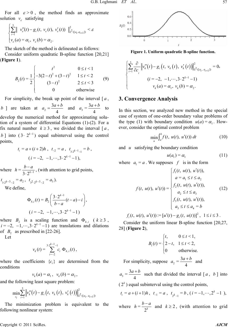 G.B. Loghmani ET AL. 57 For all >0 , the method finds an approximate solution v satisfying 322([ ,]) 1 =1 12 ()(, (), ())< ()=, ()=. iLaa ii i vtgtvt vt va vb The sketch of the method is delineated as follows: Consider uniform quadratic B-spline function [20,21] (Figure 1). 2 22 22 0<1 3(2)(3)1< 2 1 ()=2(3)2< 3 0other tt ttt Bt tt wise (9) For simplicity, the break up point of the interval [, ] are taken at a b23 4 ab a and 33 =4 ab a to develop the numerical method for approximating solu- tion of a system of differential Equations (1)-(2). For a fix natural number , we divided the interval [, ] into () equal subinterval using the control points, 3ka b31 2k =(2) i tai h =2,i , , , (), 2=ta 1,,3 1 321 = k tb 11 2 k where 1 =32 k ba h , (with attenti on t o gri d points, , ). 32 322 = k ta 23 32 2 = k ta 3 We define, 1 ,2 32 ()=( ) k ki tB tai ba ki , () 1 =2, 1,,321 k i where is a scaling function and , ki (, ) are translations and dilations of as prescribed in [22-26]. 2 B , 1 3k 1 =2,,321 k i B2 Let 1 32 1 , =2 ()= () k ki i vtc t , where the coefficients are determined from the conditions {} i c 1 ()= k va , 2 ()= k vb , and the following least square problem: 32 2([, ]) 1 =1 , , min kikk Laa cii i i vtgtvtvt The minimization problem is equivalent to the following nonlinear system: Figure 1. Uniform quadratic B-spline function. 32 2([, ]) 1 =1 1 12 , , =0 (=2, 1,,321) ()=, ()=. kikk Laa ii ii k kk vtgtvtvt c i va vb , 3. Convergence Analysis In this section, we analyzed new method in the special case of system of one-order boundary value problems of the type (1) with boundary condition 1 ()=ua . How- ever, consider the optimal control problem (, (), ()) min b a u tutut dt (10) and satisfying the boundary condition u 1 ()=ua 1 (11) where . We supp oses 1=aa is in the form 1 12 2 23 3 34 (, (), ()), = (, (), ()), (, (), ())= (, (), ()), = ftut ut aa ta ftutut ftututata ftut ut atab (12) 2 (, (), ()):=[()(, ())] ii tut ututgtut , 13i . Consider the uniform linear B-spline function [20,27, 28] (Figure 2), 1 ,0<1 ()= 2,1<2, 0otherwis tt Btt t , e. For simplicity, suppose 23 =4 ab a and 33 =4 ab a such that divided the interval [, ] into () equal subinterval using the control points, ab 2k =(1) i tai h , , , (), 1=ta 21 = k tb =1,,21 k i where =2k ba h and , (with attention to grid 2k Copyright © 2011 SciRes. AJCM  58 G.B. Loghmani ET AL. Figure 2. Uniform linear B-spline function (hat function). points, , ). 22 21 = k ta 21 k 23 321 = k ta Let , where , =1 ()= () ik i i utc t ,1 ():= ki tB 2()ta i =1, 0,i k ba, . ( 1, 2,,2 1 k ,ki 's are translations and dilations of linear spline (hat function) . 1 B Then (2)(2) 21 21 2' 1, , =1 =1 (2)(2) 32 132 1 3' 2, , 2(2) (2) =2 1=2 1 2 3 3(2) =3 21 (, (), ())= (, (), ()) (, (), ()) (, b a kk a iki iki aii kk a iki iki akk ii k b ak i ftut ut dt ftctct dt tct ctd ft 121 ' ,, (2) =3 21 (), ()) k iki iki k i ct ct t dt d (13) Furthermore, we know that the support of uniform -degree B-splines , () are into the [,] (Remark that hat functions is 1 ). On the other hand, for all fix value of , just consecutive terms of the sequence of is nonzer o. Then, we have for : dth 0 1 =B d Bt () j d Bt 1=0, 1, ,(1)j t1 {, () d Bt 2k j , } jd B 01 (), dd B, () t , (2) 2 , 23 (2) (2) , (2) 3 () 0, [, ], 221, () 0, [, ], 122 and 3221, () 0, [, ], 1322. ki kk ki kkk ki k t taa i t taa ii t tab i So, from (13), we obtain 32121 1' ,, =1=1= 1 101 21 (, (), ()) =(, (), ()) =(, , ,,) b a kk ajjikiiki aj ji i k ftut ut dt tc t c td Fcc cc t 1 (14) Therefore, in view of (14), the optimal problem (10)-(11) reduces to the problem 101 21 , , ,..., 10 121 (, , ,, ) min k cccc k Fcc cc (15) subject to 1 =()=ua c . (16) For finding , ,…, , we have to solve the system 0 c1 c21 k c =0 j F c k* , () Let =0, ,2 1j1 c , , * 0 c ** 121 ,, k cc be an approximate solution of (15)-(16) and set 21 ** , =1 ()= () k kik i utc t i . (17) We assume integral operator define the following by the form L ():=(, (), ()) b a Luf tututdt * . suppose that there exists a solution of (10) satisfying (11). (We assume .) M. Ahmadinia and G. B. Loghmani [21] shows that under reasonable conditions, converges to as . ([, ])uCab * ()Lu * ()Lu * () k Lu k Theorem. Let in (12) have the property that for all >0 there exists >0 such that |(, , ) tuv 11 (, , u v)|<ft , whenever 1 ||<uu and 1 ||<vv . Let be a exact solution of the problem: (10)-(11). Assume is continuous on [, ]. The following assertions are true. * uC b ([ ,a ]b)u*' () a 1) For all >0 there exists and k such that 2kh * )(Lu0()< k Lh , and satisfies (11). k h 2) Let be as in (17). Then and as k. * uk () k ** ( () kk Lu Lh()Lu) ** ()Lu Lu Proof. see [21]. The above theorem shows that for all >0 there exists an approximate solution for the optimal control problem (10)-(11) such that the difference between the value of and the value is at most * k u * () k Lu * (Lu) . Following the steps of the proof of above theorem we obtain the following corollary. Corollary 1. All derivatives of the approximate solution converges to the related derivatives of the exact solution. Remark 1. If the problem involves the higher derivative u B, we will use the uniform quadratic spline function 2 in (9). Here, 2 is a left continuous step function. In this method, d B ised when the regularity of d B is minial. That is, if the problem involves u B us m only, thed B n (1d ) st be chosen to be a step function; if it involves u mu and u, then d B (d2 ) Copyright © 2011 SciRes. AJCM 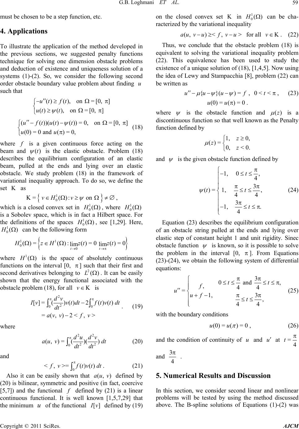 G.B. Loghmani ET AL. 59 ust b ] me chosen to be a step function, etc. 4. Applications To illustrate the application of the method developed in the previous sections, we suggested penalty functions technique for solving one dimension obstacle problems and deduction of existence and uniqueness solution of a systems (1)-(2). So, we consider the following second order obstacle boundary value problem about finding such that u ()(),on =[0, ] ()(),on =[0, ] ut ft ut t (())(()())=0,on =[0, (0)=0 and ()=0, uftut t uu (18) where is a given continuous force acting on the beam and ()t is the elastic obstacle. Problem (18) describes the equilibrium configuration of an elastic beam, pulled at the ends and lying over an elastic obstacle. We study problem (18) in the framework of variational inequality approach. To do so, we define the set as K 1 0 K= () : on vH v 1()H , which is a closed convex set in 0, where 1 0()H is a Sobolev space, which is in fact a Hilbert space. For the definitions of the spaces , see [1,29]. Here, can be the following form 1 0()H 1 0()H 11 00 ()=():()=0 ()=0 lim lim tt HzHzt zt where is the space of absolutely continuous functions on the interval [0, 1()H ] such that their first and second derivatives belonging to . It can be easily shown that the energy functional associated with the obstacle problem (18), for all is 2()L Kv 2 2 00 []= ()()2()() =(, )2<, > dv vvtdtftv dt av vfv tdt . (19) where 22 22 0 (, )=()() du dv au vdt dt dt (20) and 0 <, >=()() vftvt (,au dt . (21) Also it can be easily shown that defined by (20) is bilinear, symmetric and positive (in fact, coercive [5,7]) and the functional )v defined by (21) is a linear continuous functional. It is well known [1,5,7,29] that th e m i n i mum of the functional u[] v defined by (19) on the closed convex set in can be cha- racterized by the variational inequality K v 1 0()H (, )<,>au vufu for all . (22) Kv Thus, we conclude that the obstacle problem (18) is equivalent to solving the variational inequality problem (22). This equivalence has been used to study the existence of a unique solution of (18), [1,4,5]. Now using the idea of Lewy and Stampacchia [8], problem (22) can be written as {} )uu(u=f , 0<t< , (23) (0) ==()uu0. where is the obstacle function and ()z is a discontinuous function so that well known as the Penalty function defined by 1, 0, 0, 0. ()= < z zz and is the given obstacle function defined by 1, , 1, t 0 , 4 3 ()= 1, 44 3. 4 t t t (24) Equation (23) describes the equilibrium configuration of an obstacle string pulled at the ends and lying over elastic step of constant height 1 and unit rigidity. Sinec obstacle function is known, so it is possible to solve the problem in the interval [0, ]. From Equations (23)-(24), we obtain the following system of differential equations: 3 0 and ,44 =1,3 , 44 tt f uuf t , (25) with the boundary conditions (0) =) = 0(uu , (26) and the condition of continuity of and uu at =4 t and 3 4 . 5. Numerical Results and Discussion In this section, we consider second linear and nonlinear problems will be tested by using the method discussed above. The B-spline solutions of Equations (1)-(2) was Copyright © 2011 SciRes. AJCM  60 G.B. Loghmani ET AL. obtained using a linear combination 1 32 1 * =2 ()= k ki ut , and the minimization problem was solved by Maple 12. The least square errors (LSE) in the analytical solutions for test prob lem 1, 2 and 3 were calculated and are depicted in Tables 1-3. *, () iki ct Test problem 1 ([3,17 - 19 ], E xa mpl e 1). Consider the linear system of differential Equations (25)-(26) when , takes the following form: ()=0ft 3 0,0 and , 44 =3 1, , 44 tt u ut (27) with boundary condition (26). The analytical solution for this problem is given by 1 4 ()=, 0, 4 t ut t 2 1 4cosh( )3 2 1, 44 ()= 4( )3 , , 4 tt ut tt , (28) where 1:=4coth( ) 4 and 21 :=sinh( ) 4 . The problem (27) was solved using the mehtod described in Section 2 and 3 with a variety of values with respect to . The observed least square errors (LSE) are depicted in Table 1. We use the method and obtain this results; h 3k Approximate solution for : * k u=3k * 33,23,1 3,0 3,1 3,2 3,3 3,43,5 3,6 3,7 3,8 3,9 ( )0.05662( )0.05662( ) 0.16985()0.28308( )0.39629( ) 0.46765( )0.50213()0.50213( ) 0.46765( )0.39629( )0.28308( ) 0.16985()(0.56617 utt t tt tt tt te 3,10 3,11 1)( ) (0.566171)( ) t et t t t t t t . Approximate solution for : * k u= 4k * 44,24,1 4,0 4,1 4,2 4,3 4,4 4,54,6 4,7 4,8 4,9 ( )=0.02832( )0.02832() (0.849741)( )0.14162( ) 0.19827( )0.25492( )0.31157() 0.36821( )0.41400( )0.44972() 0.47599( )0.49325( )0.501 uttt ett tt tt tt 4,10 4,11 4,124,13 81( ) 0.50181( )0.49325()0.47599() t tt Table 1. Least square error (LSE) for Test problem 1. *() () j k uLES ()=3kLES () =4kLES () =5kLES ()=6k =0j1.6575 7e 1.65757e 5.6080 10e 1.1997 10e =1 2.4876 6e 1.57487e 9.8946 9e 8.4401 10e =2j5.0502 4e 1.2968 4e 3.2325 5e 8.0904 6e 4,14 4,15 4,16 4,174,18 4,19 4,20 4,21 3,22 3,23 0.44972()0.41400()0.31157( ) 0.25492( )0.19827()0.14162() 0.36821()(0.849741)( ) (0.283251)( )(0.283251)( ) tt tt tet et et t t . The approximate solution can also be obtained for 5, 6k . We would like to emphasize that the present method has the advantage of the ability of approximating the derivatives of u and u on [, ] where as other parametric spline and finite difference methods [2,17] do not have this ability. Mach as, cubic spline method [3] has the ability of approximating the first derivative, but it hasn't the ability of approximating the second derivatives ab such that the our method can be approximating both of first and second derivatives. Test problem 2. Consider the system of differential Equations (25)-(26) when , takes the following form: ()=2ft 3 2,0 and , 44 =3 1, , 44 tt u ut (29) with boundary condition (25). The analytical solution for this problem is given by 2 2 2 2 2 (16)sinh() 4, 42 0, 4 (16) 1cosh(), 42 ()= 3 , 44 (16)sinh( ) 4() 42 (3), 2 tt t t ut t tt t (30) Copyright © 2011 SciRes. AJCM  G.B. Loghmani ET AL. 61 3 ()= , 4 ut t where :=sinh( )4cosh( ) 44 . The problem (29) was solved using the mehtod described in Section 2 and 3 with a variety of values with respect to . The observed least square errors (LSE) are depicted in Table 2. We use the method and obtain this results; h 3k Approximate solution for : * k u=3k * 33,23,1 3,0 3,13,2 3,3 3,43,5 3,63,7 3,8 3,9 3, ( )=0.22731()0.22731( ) 0.54485()0.72531( )0.76869( ) 0.79603( )0.80924( )0.80924() 0.79603()0.76869( )0.72531( ) 0.54485()0.22731 utt t tt tt tt t 10 3,11 ( )0.22731( )t t t t t . The approximate solution can also be obtained for . 4, 5, 6k Test problem 3 ([29], Example). Consider the system of differential equation: 1 0, 04 1 1, 44 3 0, 1 4 t uut t 3 (31) with boundary conditions, (0)= (0)=(1)0uu u . The analytical solution for this problem is given by 2 1 2 2 234 56 1,1 20, 4 113 () , 33 44 cossin , 22 31 , 1(2),4 t at t ae ut t eata t t att a (32) We can find the constants , by solving a system of linear equations constructed by applying the conitinuity conditions of , i a1, 2,,6i uu , u at 1 4 t and 3 4 t. We consider , , 0.24391 i a0.17847 i a i a , , , 0.818930.30266 i a 0.24213 i a i a . 0.65376 Table 2. Least square error (LSE) for test problem 2. *() () j k uLES (=3k)LES (=4k) LES (=5k) LES (=6k) =0j2.4377 8e 1.5765 9e 4.93041e 1.366710e =1j3.6519 7e 2.313 3 8e1.5552 9e6.377501e =2j7.4138 5e 1.8891 5e 4.7577 6e 1.1897 6e Table 3. Least square error (LE) for test poblem 3. Sr *() (j k u)LES (=3k)LES (=4k) LES (=5k) LES (=6k) =0 3.3013 13e j 2.0636 14e 1.293115e 7.99371e7 =1 4.0337 12e 2.51583 1e1e1e1.57144 9.8027 6 =2j2.4877 10e 1.5545 11e9.7153 13e6.0670 14e =3j1.0822 6e 2.70417e 6.75938e 1.6897 8e using the mehtod described in Section 2 and 3 with a variety of values with respect to . The et ociated with the three examples discussed above were performed by using Maple 12. Co dgements ous reviewers for their helpful comments, which greatly improves this erences nd J. T. Oden, “Contact Problems in IAM Publishing Company, Philadelphia, es for Solving Obstacle Problems,” Applied h3k observed least square errors (LSE) are given in Table 3. We use the mhod and obtain this results. 6. Conclusions The computations ass mparing the obtained results with other works [3,13, 16-19], this method was clearly reliable if compared with grid points techniques where solution is defined at grid points only. Moreover the method yields a good result even for small k. 7. Acknowle The authors are grateful to the anonym paper. 8. Ref [1] N. Kikuchi a Elasticity,” S 1988. [2] M. A. Noor and S. I. A. Tirmizi, “Finite Difference Techniqu Mathematics Letters, Vol. 1, No. 3, 1988, pp. 267-271. doi:10.1016/0893-9659(88)90090-0 [3] E. A. Al-Said, “ The Use of Cubic Splines in the Nu- merical Solution of a System of Seco nd Order Boundary Value Problems,” Computers & Mathematics with Appli- cations, Vol. 42, No. 6, September 2001, pp. 861-869. doi:10.1016/S0898-1221(01)00204-8 [4] C. Baiocchi and A. Capelo, “Variational and Quas -Variational Inequalities,” John Willei- y and Sons, New Problems,” John Willey and Sons, New York, 1982. York, 1984. [5] A. Friedman, “Variational Principles and Free-Boundary The homogeneous linear problem (31) was solved Copyright © 2011 SciRes. AJCM 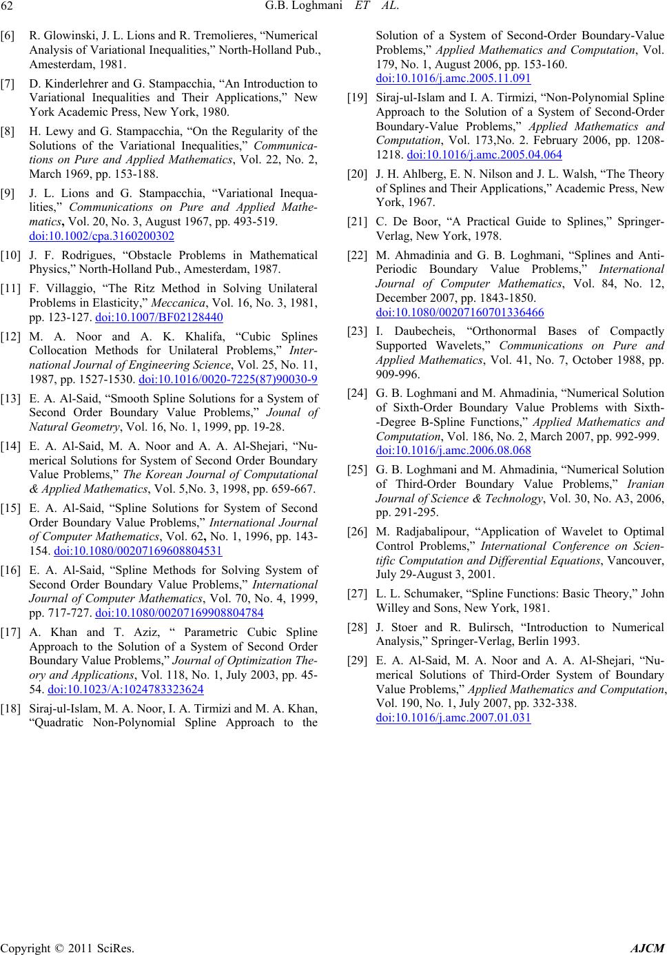 G.B. Loghmani ET AL. Copyright © 2011 SciRes. AJCM 62 . L. Lions and R. Tremolieres, “Num[6] R. Glowinski, Jerical Analysis of Variational Inequalities,” North-Holland Pub., Amesterdam, 1981. [7] D. Kinderlehrer and G. Stampacchia, “An Introduction to Variational Inequalities and Their Applications,” New York Academic Press, New York, 1980. [8] H. Lewy and G. Stampacchia, “On the Regularity of the Solutions of the Variational Inequalities,” Communica- tions on Pure and Applied Mathematics, Vol. 22, No. 2, March 1969, pp. 153-188. [9] J. L. Lions and G. Stampacchia, “Variational Inequa- lities,” Communications on Pure and Applied Mathe- matics, Vol. 20, No. 3, August 1967, pp. 493-519. doi:10.1002/cpa.3160200302 [10] J. F. Rodrigues, “Obstacle Problems in Mathematical Physics,” North-Holland Pub., Amesterdam, 1987. [11] F. Villaggio, “The Ritz Method in Solving Unilateral Problems in Elasticity,” Meccanica, Vol. 16, No. 3, 1981, pp. 123-127. doi:10.1007/BF02128440 [12] M. A. Noor and A. K. Khalifa, “Cubic Splines Collocation Methods for Unilateral Problems,” Inter- national Journal of Engineering Science, Vol. 25, No. 11, 1987, pp. 1527-1530. doi:10.1016/0020-7225(87)90030-9 [13] E. A. Al-Said, “Smooth Spline Solutions for a System of Second Order Boundary Value Problems,” Jounal of Natural Geometry, Vol. 16, No. 1, 1999, pp. 19-28. [14] E. A. Al-Said, M. A. Noor and A. A. Al-Shejari, “Nu- merical Solutions for System of Second Order Boundary Value Problems,” The Korean Journal of Computational & Applied Mathematics, Vol. 5,No. 3, 1998, pp. 659-667. [ 15] E. A. Al-Said, “Spline Solutions for System of Second Order Boundary Value Problems,” International Journal of Computer Mathematics, Vol. 62, No. 1, 1996, pp. 143- 154. doi:10.1080/00207169608804531 [16] E. A. Al-Said, “Spline Methods for Solving System of Second Order Boundary Value Problems,” International Journal of Computer Mathematics, Vol. 70, No. 4, 1999, pp. 717-727. doi:10.1080/00207169908804784 [17] A. Khan and T. Aziz, “ Parametric Cubic Spline Approach to the Solution of a System of Second Order Boundary Value Problems,” Journal of Optimization The- ory and Applications, Vol. 118, No. 1, July 2003, pp. 45- 54. doi:10.1023/A:1024783323624 [18] Siraj-ul-Islam, M. A. Noor, I. A. Tirmizi and M. A. Khan, “Quadratic Non-Polynomial Spline Approach to the Solution of a System of Second-Order Boundary-Value Problems,” Applied Mathematics and Computation, Vol. 179, No. 1, August 2006, pp. 153-160. doi:10.1016/j.amc.2005.11.091 [19] Siraj-ul-Islam and I. A. Tirmizi, “Non-Po Approach to the Solution of a lynomial Spline System of Second-Order Boundary-Value Problems,” Applied Mathematics and Computation, Vol. 173,No. 2. February 2006, pp. 1208- 1218. doi:10.1016/j.amc.2005.04.064 [20] J. H. Ahlberg, E. N. Nilson and J. L. Walsh, “The Theory of Splines and Their Applications,” Academic Press, New ork, 1978. e Problems,” International York, 1967. [21] C. De Boor, “A Practical Guide to Splines,” Springer- Verlag, New Y [22] M. Ahmadinia and G. B. Loghmani, “Splines and Anti- Periodic Boundary Valu Journal of Computer Mathematics, Vol. 84, No. 12, December 2007, pp. 1843-1850. doi:10.1080/00207160701336466 [23] I. Daubecheis, “Orthonormal Supported Wavelets,” Communic Bases of Compactly ations on Pure and der Boundary Value Problems with Sixth- Applied Mathematics, Vol. 41, No. 7, October 1988, pp. 909-996. [24] G. B. Loghmani and M. Ahmadinia, “Numerical Solution of Sixth-Or -Degree B-Spline Functions,” Applied Mathematics and Computation, Vol. 186, No. 2, March 2007, pp. 992-999. doi:10.1016/j.amc.2006.08.068 [25] G. B. Loghmani and M. Ahmadinia, “Numerical Solution of Third-Order Boundary Value Problems,” Iranian ms,” International Conference on Scien- k, 1981. 93. of Boundary Journal of Science & Technology, Vol. 30, No. A3, 2006, pp. 291-295. [26] M. Radjabalipour, “Application of Wavelet to Optimal Control Proble tific Computation and Differential Equations, Vancouver, July 29-August 3, 2001. [27] L. L. Schumaker, “Spline Functions: Basic Theory,” John Willey and Sons, New Yor [28] J. Stoer and R. Bulirsch, “Introduction to Numerical Analysis,” Springer-Verlag, Berlin 19 [29] E. A. Al-Said, M. A. Noor and A. A. Al-Shejari, “Nu- merical Solutions of Third-Order System Value Problems,” Applied Mathematics and Computation, Vol. 190, No. 1, July 2007, pp. 332-338. doi:10.1016/j.amc.2007.01.031
|