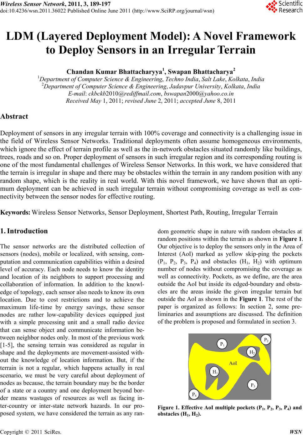
 Wireless Sensor Network, 2011, 3, 189-197 doi:10.4236/wsn.2011.36022 Published Online June 2011 (http://www.SciRP.org/journal/wsn) Copyright © 2011 SciRes. WSN LDM (Layered Deployment Model): A Novel Framework to Deploy Sensors in an Irregular Terrain Chandan Kumar Bhattacharyya1, Swapan Bhattacharya2 1Department of Computer Science & Engineering, Techno India, Salt Lake, Kolkata, India 2Department of Computer Science & Engineering, Jadavpur University, Kolkata, India E-mail: ckbckb2010@rediffmail.com, bswapan2000@yahoo.co.in Received May 1, 2011; revised June 2, 2011; accepted June 8, 2011 Abstract Deployment of sensors in any irregular terrain with 100% coverage and connectivity is a challenging issue in the field of Wireless Sensor Networks. Traditional deployments often assume homogeneous environments, which ignore the effect of terrain profile as well as the in-network obstacles situated randomly like buildings, trees, roads and so on. Proper deployment of sensors in such irregular region and its corresponding routing is one of the most fundamental challenges of Wireless Sensor Networks. In this work, we have considered that the terrain is irregular in shape and there may be obstacles within the terrain in any random position with any random shape, which is the reality in real world. With this novel framework, we have shown that an opti- mum deployment can be achieved in such irregular terrain without compromising coverage as well as con- nectivity between the sensor nodes for effective routing. Keywords: Wireless Sensor Networks, Sensor Deployment, Shortest Path, Routing, Irregular Terrain 1. Introduction The sensor networks are the distributed collection of sensors (nodes), mobile or localized, with sensing, com- putation and co mmunication capabilities with in a desired level of accuracy. Each node needs to know the identity and location of its neighbors to support processing and collaboration of information. In addition to the knowl- edge of topology, each sensor also needs to know its own location. Due to cost restrictions and to achieve the maximum life-time by energy savings, these sensor nodes are rather low-capability devices equipped just with a simple processing unit and a small radio device that can sense object and communicate information be- tween neighbor nodes on ly. In most of the previous work [1-5], the sensing terrain was considered as regular in shape and the deployments are movement-assisted with- out the knowledge of location information. But, if the terrain is not a regular, which happens actually in real scenario, we must be very careful about deployment of nodes as because, the terrain boundary may be the border of a state or a country and one deployment beyond bor- der means wastages of resources as well as facing in- ter-country or inter-state network hazards. In our pro- posed system, we have considered the terrain as any ran- dom geometric shape in nature with random obstacles at random positions within th e terrain as shown in Figure 1. Our objective is to deploy the sensors only in the Area of Interest (AoI) marked as yellow skip-ping the pockets (P1, P2, P3, P4) and obstacles (H1, H2) with optimum number of nodes without compromising the coverage as well as connectivity. Pockets, as we define, are the area outside the AoI but inside its edged-boundary and obsta- cles are the areas inside the given irregular terrain but outside the AoI as shown in the Figure 1. The rest of the paper is organized as follows: In section 2, some pre- liminaries and assumptions are discussed. The definition of the problem is proposed and formulated in section 3. Figure 1. Effective AoI multiple pockets (P1, P2, P3, P4) and obstacles (H1, H2).  190 C. K. BHATTACHARYYA ET AL. In section 4, we briefly discuss the related work. Section 5 and 6 is our proposal for the topology of node deploy- ment in LDM framework and corresponding routing methodology respectively. A simulated study of this so- lution is given in section 7. Finally, we conclude in sec- tion 8. 2. Preliminaries and Assumptions The proper sensing of any object by a sensor is highly related with the geometric distance of the object from the sensor. Here we assume that a sensor can sense the en- ergy emitted by the object in a homogeneous circular area with maximum radius r, as shown in Figure 2, un- der the constraint of noise and other distortions. This energy is called Threshold Energy (Eth) and an object will not be sensed if the received energy by the sensor is less than this threshold energy. This coverage is consid- ered as optimum coverage of a sensor with desired level of acceptable value. Assuming the energy emitted by an object is constant, the signal energy Es, as detected by sensor si for an object situated at distance dt from the sensor will be, Es = E0(1-αdn) where E0 is the energy at distance 0 i.e. maximum energy, α is the decay co-efficient and dn is the normalized distance of the ob- ject from the sensor and will be expressed as dn = dt/r where r is the optimum sensing range. For example, in the Figure 2, the signal energies for three different loca- tions ar e expressed as: Eth = E0(1 – α) = Threshold Energy; Ex = E0(1 – αdx/r) = Energy at distance dx; Ey = E0(1 – αdy/r) = Energy at distance dy. Since dx > dy, it is obviously Ex < Ey. An object will be sensed only if its emitted energy lies between E0 and Eth. We assume that the wireless sensor nodes are given as a set S with n sensor nodes where 1jni and for each sensor si, its location iii SS )y(,lx is known as it is deployed. We also assume that all the sensors are static sensors and there are no road constraints within AoI. Each sensor is assumed to have same sensing range as Figure 2. Measurement of signal energy with respect to the distance. denoted by r. A pair of sensors will be able to see (cov- erage) and hear (connectivity) each other if they have overlapped coverage space. If only coverage is consid- ered, less number of nodes will be required but the de- ployed nodes will not be able to communicate with each other. Figure 3 shows the relation between the optimal coverage and connectivity. As we move from coverage to connectivity, the overlapping domain (d) gets in- creased where ,dfr . Here, we assume homoge- neous coverage and connectivity i.e. both coverage and connectivity ranges are same and is equal to r. 3. Problem Definition and Objectives To communicate between each other with optimum cov- erage we have to deploy the next node at the maximum sensing boundary with threshold signal energy Eth to any of the four sides (i.e. Right, Left, Up, Down) of the pre- viously deployed. To minimize the channel overhead, we have proposed the concept of layered accumulation i.e. outer layer information will only be transmitted to its immediate inner layer and not directly to Fusion Node and communication to Fusion Node will be done only through First layer nodes (and/or from the boundary nodes for leaving of any object from AoI). Since volume of information is being increased layer by layer towards the Fusion Node, we have deployed nodes with variable capacities in different layers. We define capacity of a node as its rate of consumption of power, maximum sto- rage/buffer size, processing speed etc. Hence, the objec- tive or the pr oblem definition of our proposed model can be defined as: Finding Fusion Node Capacity Deploying Layer wise Sensors with variable capaci- ties Designing Effective Routing Model 4. Related Work Several deployment schemes with existing holes [7-9] in the network have been proposed to enhance the coverage. They have considered that the target region is regular and rectangular and the holes are situated randomly within Figure 3. Moving from coverage to connectivity. Copyright © 2011 SciRes. WSN  C. K. BHATTACHARYYA ET AL. Copyright © 2011 SciRes. WSN 191 Table 1. Comparative analysis of existing work with proposed model. Studies Coverage Density Full Coverage Boundary In-boundary Obstacle Obstacle Information Boundary Nodes Detected Knowledge of Neighbor Location Shortest P ath [10] Non-UniformNo Irregular Not Exist Not KnownNo Not KnownNot Known [11] Non-UniformNo Irregular Not Exist Not KnownNo Not KnownNot Known [12] Non-UniformNo Irregular Not Exist Not KnownNo Not KnownNot Known [13] Uniform Yes Irregular Not Exist Not KnownNo Not KnownNot Known [14] Non-UniformNo Irregular Not Exist Not KnownNo Not KnownNot Known [15] Non-UniformNo Irregular Not Exist Not KnownNo Not KnownNot Known LDM (Proposed) Uniform Yes Irregular Exist and Irregular Not KnownYes Known Known 5. Proposed Model the target boundary. More over the geometry of the ho les are also bounded and ar e defined as a regular graph with certain number of nodes and edges. In certain cases, holes defined with less than four edges could turn out to be large areas that act as greater barriers to the network than normal. An extreme scenario could present itself with the occurrence of a large area that is only connected through two edges. With such consideration, we need to deploy more nodes to cover the entire range of area, which is a trade-off with cost optimization. In [10-15], irregular areas have been considered with no obstacles. A comparative analysis is shown in Table 1 with proposed model. Let us define our proposed model i.e. Layered Deploy- ment Model (LDM). If a logical grid is created around a deployed node, some part of the grid area remains un- covered as shown in the Figure 4. The uncovered area will further be covered with next layer of deployment at distance r from the deployed node at right, left, up and down subject to the calculated co-ordinates of deploy- ment lie within AoI, otherwise we have to search for next effective location in any of the four sides at distance r and establish connectivity. The stepwise deployment of five nodes is shown in the Figure 5 and corresponding maximum coverage area with optimum connectivity is shown in the Figure 6. Figure 7 shows the final model The accuracy of sensor placement may be subject to various errors. Kenan Xu, et al. [16], in their paper, iden- tified two deployment errors namely, misalignment and random errors. They derived the minimum number of sensors required by a robust grid-based sensor deploy- ment assuming that the errors are bounded. F. Zhao, et al. [17], have addressed the dynamic sensor collaboration problem to determine dynamically which sensor is most appropriate to perform the sensing, what needs to be sensed, and to whom to communicate the information. It is based on the information-driven sensor querying ap- proach, enabling collaboration, under resource con- straints and cost of transmitting information. Here, the next node selection is done by predicting Mahalanobis distance measure technique where the computation from predicted likelihood function may be strongly biased by the prior distribution. Y. Rachlin, R. Negi, and P. Khosla, [18] have addressed the technique of measuring sensing capacity in a sensor network with respect to the maxi- mum ratio of target positions to sensors as achievable within a certain tolerable distortion. As one target is be- ing sensed by more than one sensor, the network will soon get flooded with redundant information. Moreover, sensors lifetime will eventually get reduced as all the time more than one sensor is sensing one target. [19,20] [21] are based on grid-based Stable Routing Protocol with multi-hop broadcast technique. In [22] several power-efficient routing algorithms are proposed for a sensor network with 2D gri d top olo gy . Figure 4. Logical grid with covered and uncovered area for a node deployed. Figure 5. Stepwise deployment of five nodes (one central and four neighbors) at right, le ft, up and down respectively. 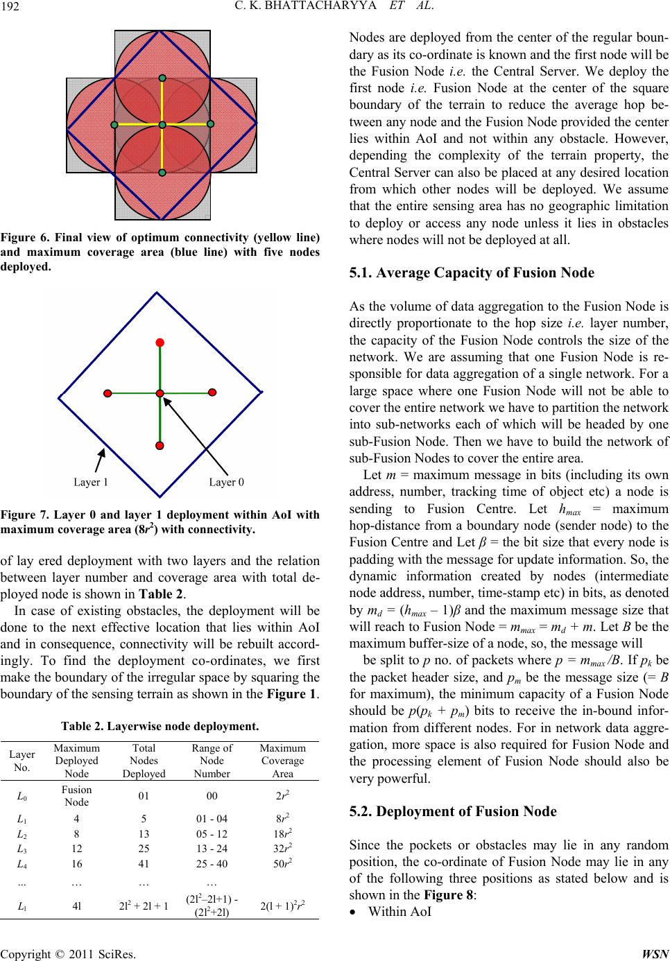 192 C. K. BHATTACHARYYA ET AL. Figure 6. Final view of optimum connectivity (yellow line) and maximum coverage area (blue line) with five nodes deployed. Figure 7. Layer 0 and layer 1 deployment within AoI with maximum coverage area (8r2) with connectivit y. of lay ered deployment with two layers and the relation between layer number and coverage area with total de- ployed node is shown in Table 2. In case of existing obstacles, the deployment will be done to the next effective location that lies within AoI and in consequence, connectivity will be rebuilt accord- ingly. To find the deployment co-ordinates, we first make the boundary of the irregular space by squaring the boundary of the sensing terrain as shown in the Figure 1. Table 2. Layerwise node de ployment. Layer No. Maximum Deployed Node Total Nodes Deployed Range of Node Number Maximum Coverage Area L0 Fusion Node 01 00 2r2 L1 4 5 01 - 04 8r2 L2 8 13 05 - 12 18r2 L3 12 25 13 - 24 32r2 L4 16 41 25 - 40 50r2 ... … … … Ll 4l 2l2 + 2l + 1(2l2–2l+1) - (2l2+2l) 2(l + 1)2r2 Nodes are deployed from the center of the regular boun- dary as its co-ordinate is known and the first node will be the Fusion Node i.e. the Central Server. We deploy the first node i.e. Fusion Node at the center of the square boundary of the terrain to reduce the average hop be- tween any node and the Fusion Node provided the center lies within AoI and not within any obstacle. However, depending the complexity of the terrain property, the Central Server can also be placed at any desired location from which other nodes will be deployed. We assume that the entire sensing area has no geographic limitation to deploy or access any node unless it lies in obstacles where nodes will not be deployed at all. 5.1. Average Capacity of Fusion Node As the volume of data aggregation to the Fusion Node is directly proportionate to the hop size i.e. layer number, the capacity of the Fusion Node controls the size of the network. We are assuming that one Fusion Node is re- sponsible for data ag gregation of a single network. For a large space where one Fusion Node will not be able to cover the entire network we have to partition the network into sub-networks each of which will be headed by one sub-Fusion Node. Then we have to build the network of sub-Fusion Nodes to cover the entire area. Let m = maximum message in bits (including its own address, number, tracking time of object etc) a node is sending to Fusion Centre. Let hmax = maximum hop-distance from a boundary node (sender node) to the Fusion Centre and Let β = the bit size that every node is padding with the message for update information. So, the dynamic information created by nodes (intermediate node address, number, time-stamp etc) in bits, as denoted by md = (hmax – 1)β and the maximum message size that will reach to Fusion Node = mmax = md + m. Let B be the maximum buffer-size of a node, so, the message will be split to p no. of packets where p = mmax /B. If pk be the packet header size, and pm be the message size (= B for maximum), the minimum capacity of a Fusion Node should be p(pk + pm) bits to receive the in-bound infor- mation from different nodes. For in network data aggre- gation, more space is also required for Fusion Node and the processing element of Fusion Node should also be very powerful. 5.2. Deployment of Fusion Node Since the pockets or obstacles may lie in any random position, the co-ordinate of Fusion Node may lie in any of the following three positions as stated below and is shown in the Figure 8: Withi n AoI Copyright © 2011 SciRes. WSN 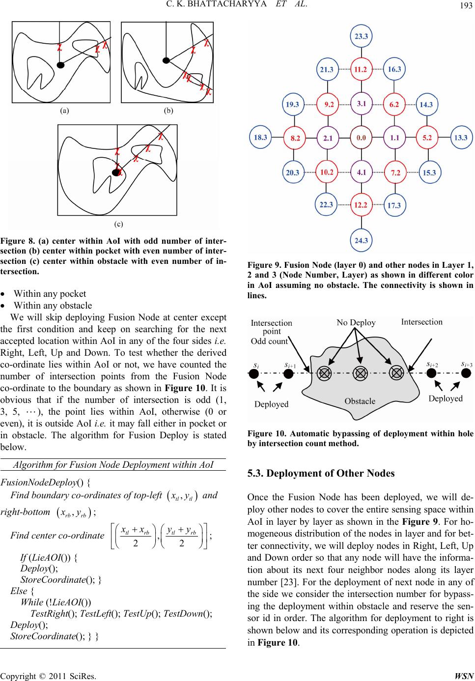 C. K. BHATTACHARYYA ET AL. 193 Figure 8. (a) center within AoI with odd number of inter- section (b) center within pocket with even number of inter- section (c) center within obstacle with even number of in- tersection. Within any pocket Within any obstacle We will skip deploying Fusion Node at center except the first condition and keep on searching for the next accepted location within AoI in any of the four sides i.e. Right, Left, Up and Down. To test whether the derived co-ordinate lies within AoI or not, we have counted the number of intersection points from the Fusion Node co-ordinate to the boundary as shown in Figure 10. It is obvious that if the number of intersection is odd (1, 3, 5, ), the point lies within AoI, otherwise (0 or even), it is outside AoI i.e. it may fall either in pocket or in obstacle. The algorithm for Fusion Deploy is stated below. Algorithm for Fusion Node Deployment within AoI FusionNodeDeploy() { Find boundary co-ordinates of top-left , tl tl y and right-bottom , rb rb y; Find center co-ordinate , 22 tl rbtlrb xx yy Figure 9. Fusion Node (layer 0) and other nodes in Layer 1, 2 and 3 (Node Number, Layer) as shown in different color in AoI assuming no obstacle. The connectivity is shown in lines. Figure 10. Automatic bypassing of deployment within hole by intersection count method. 5.3. Deployment of Other Nodes ; If (LieAOI()) { Deploy(); StoreCoordinate(); } Else { While (!LieAOI()) TestRight(); TestLeft(); TestUp(); TestDown(); Deploy(); StoreCoordinate(); } } Once the Fusion Node has been deployed, we will de- ploy other nodes to cover the entire sensing space within AoI in layer by layer as shown in the Figure 9. For ho- mogeneous distribution of the nodes in layer and for bet- ter connectivity, we will deploy nodes in Right, Left, Up and Down order so that any node will have the informa- tion about its next four neighbor nodes along its layer number [23]. For the deployment of next node in any of the side we consider the intersection number for bypass- ing the deployment within obstacle and reserve the sen- sor id in order. The algorithm for deployment to right is shown below and its corresponding operation is depicted in Figure 10. Copyright © 2011 SciRes. WSN 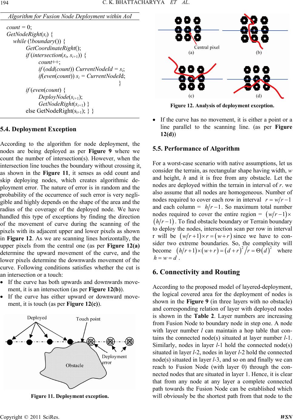 194 C. K. BHATTACHARYYA ET AL. Algorithm for Fusion Node Deployment within AoI count = 0; GetNodeRight(si) { while (!boundary()) { GetCoordinateRight(); if (intersection(si, si+1)) { count++; if (odd(count)) CurrentNodeId = si; if(even(count)) si = CurrentNodeId; } if (even(count) { DeployNode(si+1); GetNodeRight(si+1) } else GetNodeRight(si+1); } } 5.4. Deployment Exception According to the algorithm for node deployment, the nodes are being deployed as per Figure 9 where we count the number of intersection(s). However, when the intersection line touches the boundary without crossin g it, as shown in the Figure 11, it senses as odd count and skip deploying nodes, which creates algorithmic de- ployment error. The nature of error is in random and the probability of the occurrence of such error is very negli- gible and highly depends on the shape of the area and the radius of the coverage of the deployed node. We have handled this type of exceptions by finding the direction of the movement of curve during the scanning of the pixels with its adjacent upper and lower pixels as shown in Figure 12. As we are scanning lines horizontally, the upper pixels from the central one (as per Figure 12(a) determine the upward movement of the curve, and the lower pixels determine the downwards movement of the curve. Following conditions satisfies whether the cut is an intersection or a touch: If the curve has both upwards and downwards move- ment, it is an intersection (as per Figure 12(b)). If the curve has either upward or downward move- ment, it is touch (as per Figure 12(c)). Figure 11. Deployme nt exception. Figure 12. Analysis of deployment exception. If the curve has no movement, it is either a point or a line parallel to the scanning line. (as per Figure 12(d)) 5.5. Performance of Algorithm For a worst-case scenario with native assumptions, let us consider the terrain, as rectangular shape having width, w and height, h and it is free from any obstacle. Let the nodes are deployed within the terrain in interval of r. we also assume that all nodes are homogeneous. Number of nodes required to cover each row in interval 1rwr and each column = 1hr . So maximum total number nodes required to cover the entire region = 1wr 1hr . To find obstacle boundary or Terrain boundary to deploy the nodes, intersection scan per row in interval r will be 1rw rwr since we have to con- sider two extreme boundaries. So, the complexity will become 22 w rdrrd where1hr hwd . 6. Connectivity and Routing According to the proposed model of layered-deployment, the logical covered area for the deployment of nodes is shown in the Figure 9 (in three layers with no obstacle) and corresponding relation of layer with deployed nodes is shown in the Table 2. Layer numbers are increasing from Fusion Node to boundary node in step one. A node with layer number l can maintain a hop table that con- tains the connected node(s) situated at layer number l-1. Similarly, nodes in layer l-1 hold the connected node(s) situated in layer l-2, nodes in layer l-2 hold the connected node(s) situated in layer l-3, and so on and finally we can reach to Fusion Node (with layer 0) through the con- nected nodes that are situated in layer 1. Hence, it is clear that from any node at any layer a complete connected path towards the Fusion Node can be established which will obviously be the shortest path from that node to the Copyright © 2011 SciRes. WSN 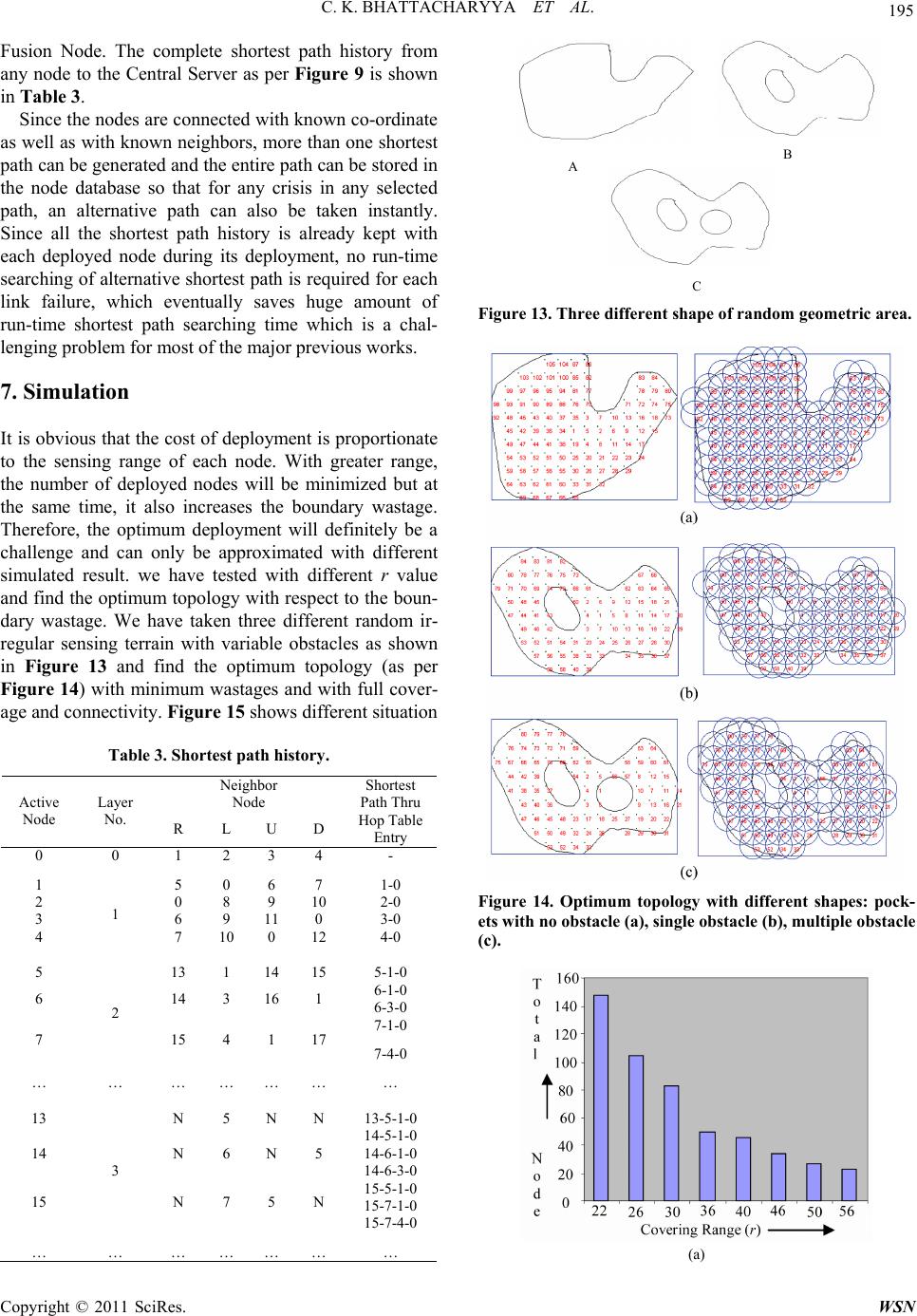 C. K. BHATTACHARYYA ET AL. 195 Fusion Node. The complete shortest path history from any node to the Central Server as per Figure 9 is shown in Table 3. Since the nodes are connected with known co-ordinate as well as with known neighbors, more than one shortest path can be generated and the entire path can be stored in the node database so that for any crisis in any selected path, an alternative path can also be taken instantly. Since all the shortest path history is already kept with each deployed node during its deployment, no run-time searching of alternative shortest path is required for each link failure, which eventually saves huge amount of run-time shortest path searching time which is a chal- lenging problem for most of the major previous works. 7. Simulation It is obvious that the cost of deployment is proportionate to the sensing range of each node. With greater range, the number of deployed nodes will be minimized but at the same time, it also increases the boundary wastage. Therefore, the optimum deployment will definitely be a challenge and can only be approximated with different simulated result. we have tested with different r value and find the optimum topology with respect to the boun- dary wastage. We have taken three different random ir- regular sensing terrain with variable obstacles as shown in Figure 13 and find the optimum topology (as per Figure 14) with minimum wastages and with full cover- age and co nn ectiv ity. Figure 15 shows different situ atio n Table 3. Shortest path history. Neighbor Node Active Node Layer No. R L U D Shortest Path Thru Hop Table Entry 0 0 1 2 3 4 - 1 5 0 6 7 1-0 2 0 8 9 10 2-0 3 6 9 11 0 3-0 4 1 7 10 0 12 4-0 5 13 1 14 15 5-1-0 6 14 3 16 1 6-1-0 6-3-0 7 2 15 4 1 17 7-1-0 7-4-0 … … … … … … … 13 N 5 N N 13-5-1-0 14 N 6 N 5 14-5-1-0 14-6-1-0 14-6-3-0 15 3 N 7 5 N 15-5-1-0 15-7-1-0 15-7-4-0 … … … … … … … A B C Figure 13. Three different shape of random geometric area. Figure 14. Optimum topology with different shapes: pock- ets with no obstacle (a), single obstacle (b), multiple obstacle (c). (a) Copyright © 2011 SciRes. WSN 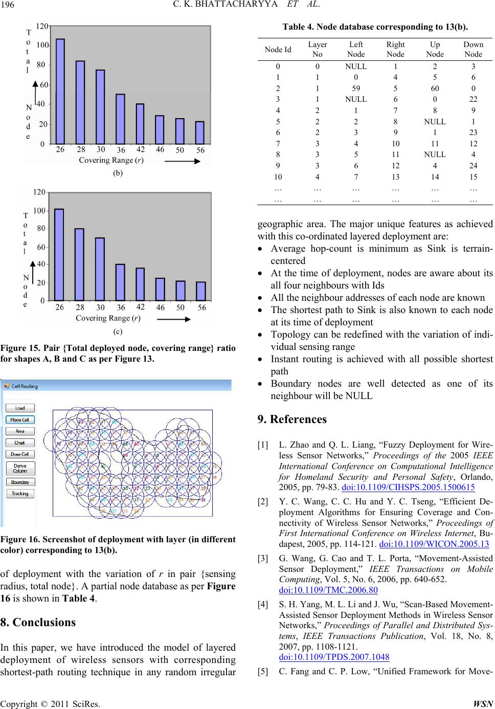 196 C. K. BHATTACHARYYA ET AL. (b) (c) Figure 15. Pair {Total deploy node, covering range}ed ratio for shapes A, B and C as per Figure 13. Figure 16. Scree nshot of deploy ment with layer (in differe n f deployment with the variation of r in pair {sensing this paper, we have introduced the model of lay deployment of wireless sensors with corresponding shortest-path routing technique in any random irregular t color) corresponding to 13(b). o radius, total node}. A partial node database as per Figure 16 is shown in Table 4. 8. Conclusions Inered Table 4. Node database corresponding to 13(b). Node IdLayer No Left Node Right Node Up Node Down Node 0 0 NULL 1 2 3 1 N 1 1 0 59 4 5 5 60 6 0 2 3 1 NULL 6 0 22 4 2 1 7 8 9 5 2 2 8 ULL1 6 2 3 9 1 23 7 3 4 10 11 12 8 3 5 11 NULL 4 9 3 6 12 4 24 10 4 7 13 14 15 … … … … … … … … … … … … geohic a The uni featuas ach with this co-ordinated red deyment are: Average hop-count is minimum as Sink is terrain- about its ighbour addresses of each node are known - d with all possible shortest well detected as one of its ] L. Zhao and Q. L. Liang, “Fuzzy Deployment for Wire- etworks,” Proceedings of the 2005 IEEE onference on Computational Intelligence grap rea.major queres ieved laye plo centered At the time of deployment, nodes are aware all four neighbours with Ids All the ne The shortest path to Sink is also known to each node at its time of deployment Topology can be redefined with the variation of indi vidual sensing range Instant routing is achieve path Boundary nodes are neighbour will be NULL 9. References [1 less Sensor N International C for Homeland Security and Personal Safety, Orlando, 2005, pp. 79-83. doi:10.1109/CIHSPS.2005.1500615 [2] Y. C. Wang, C. C. Hu and Y. C. Tseng, “Efficient De- ployment Algorithms for Ensuring Coverage and Con- nectivity of Wireless Sensor Networks,” Proceedings of First International Conference on Wireless Internet, Bu- dapest, 2005, pp. 114-121. doi:10.1109/WICON.2005.13 [3] G. Wang, G. Cao and T. L. Porta, “Movement-Assisted Sensor Deployment,” IEEE Transactions on Mobile Computing, Vol. 5, No. 6, 2006, pp. 640-652. doi:10.1109/TMC.2006.80 [4] S. H. Yang, M. L. Li and J. Wu, “Scan-Based Movement- Assisted Sensor Deployment Methods in Wire Networks,” Proceedings of less Sensor Parallel and Distributed Sys- tems, IEEE Transactions Publication, Vol. 18, No. 8, 2007, pp. 1108-1121. doi:10.1109/TPDS.2007.1048 [5] C. Fang and C. P. Low, “Unified Framework for Move- Copyright © 2011 SciRes. WSN 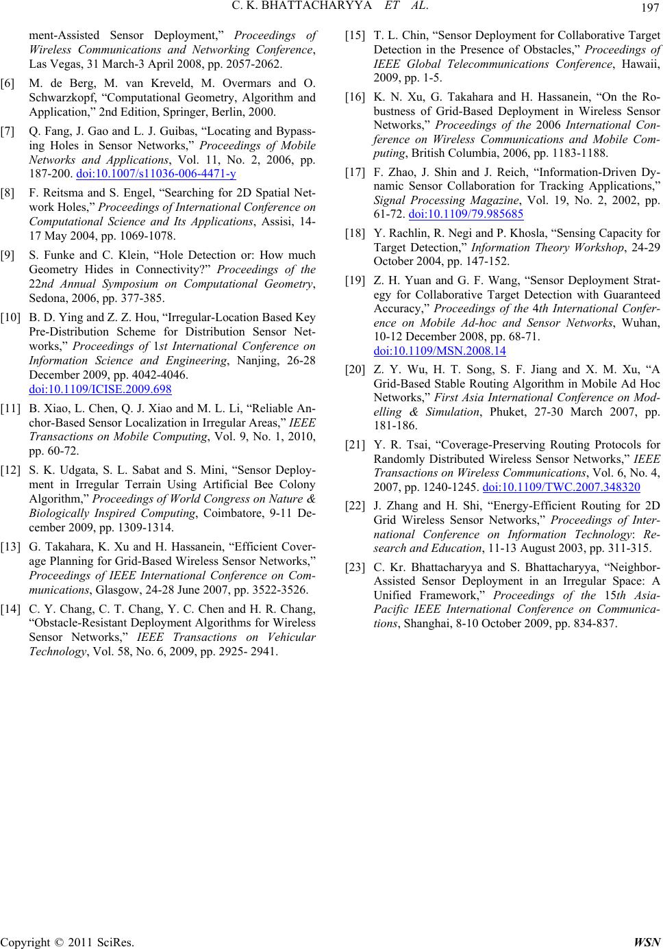 C. K. BHATTACHARYYA ET AL. Copyright © 2011 SciRes. WSN 197 Deployment,” Proceedings of Networking Conference 6, pp. ment-Assisted Sensor Wireless Communications and, Las Vegas, 31 March-3 April 2008, pp. 2057-2062. [6] M. de Berg, M. van Kreveld, M. Overmars and O. Schwarzkopf, “Computational Geometry, Algorithm and Application,” 2nd Edition, Springer, Berlin, 2000. [7] Q. Fang, J. Gao and L. J. Guibas, “Locating and Bypass- ing Holes in Sensor Networks,” Proceedings of Mobile Networks and Applications, Vol. 11, No. 2, 200 187-200. doi:10.1007/s11036-006-4471-y [8] F. Reitsma and S. Engel, “Searching for 2D Spatial Net- work Holes,” Proceedings of International Conference on Computational Science and Its Applications, Assisi, 14- Computational Geometry, International Conference on 17 May 2004, pp. 1069-1078. [9] S. Funke and C. Klein, “Hole Detection or: How much Geometry Hides in Connectivity?” Proceedings of the 22nd Annual Symposium on Sedona, 2006, pp. 377-385. [10] B. D. Ying and Z. Z. Hou, “Irregular-Location Based Key Pre-Distribution Scheme for Distribution Sensor Net- works,” Proceedings of 1st Information Science and Engineering, Nanjing, 26-28 December 2009, pp. 4042-4046. doi:10.1109/ICISE.2009.698 [11] B. Xiao, L. Chen, Q. J. Xiao and M. L. Li, “Reliable An- chor-Based Sensor Localization in Irr Transactions on Mobile Comp egular Areas,” IEEE uting, Vol. 9, No. 1, 2010, Proceedings of World Congress on Nature & ional Conference on Com- Target Takahara and H. Hassanein, “On the Ro- iven Dy- pp. 60-72. [12] S. K. Udgata, S. L. Sabat and S. Mini, “Sensor Deploy- ment in Irregular Terrain Using Artificial Bee Colony Algorithm,” Biologically Inspired Computing, Coimbatore, 9-11 De- cember 2009, pp. 1309-1314. [13] G. Takahara, K. Xu and H. Hassanein, “Efficient Cover- age Planning for Grid-Based Wireless Sensor Networks,” Proceedings of IEEE Internat munications, Glasgow, 24-28 June 2007, pp. 3522-3526. [14] C. Y. Chang, C. T. Chang, Y. C. Chen and H. R. Chang, “Obstacle-Resistant Deployment Algorithms for Wireless Sensor Networks,” IEEE Transactions on Vehicular Technology, Vol. 58, No. 6, 2009, pp. 2925- 2941. [15] T. L. Chin, “Sensor Deployment for Collaborative Detection in the Presence of Obstacles,” Proceedings of IEEE Global Telecommunications Conference, Hawaii, 2009, pp. 1-5. [16] K. N. Xu, G. bustness of Grid-Based Deployment in Wireless Sensor Networks,” Proceedings of the 2006 International Con- ference on Wireless Communications and Mobile Com- puting, British Columbia, 2006, pp. 1183-1188. [17] F. Zhao, J. Shin and J. Reich, “Information-Dr namic Sensor Collaboration for Tracking Applications,” Signal Processing Magazine, Vol. 19, No. 2, 2002, pp. 61-72. doi:10.1109/79.985685 [18] Y. Rachlin, R. Negi and P. Khosla, “Sensing Capacity for , “Sensor Deployment Strat- Target Detection,” Information Theory Workshop, 24-29 October 2004, pp. 147-152. [19] Z. H. Yuan and G. F. Wang egy for Collaborative Target Detection with Guaranteed Accuracy,” Proceedings of the 4th International Confer- ence on Mobile Ad-hoc and Sensor Networks, Wuhan, 10-12 December 2008, pp. 68-71. doi:10.1109/MSN.2008.14 [20] Z. Y. Wu, H. T. Song, S. F. Jiang and X. M. Xu, “A i, “Coverage-Preserving Routing Protocols for Grid-Based Stable Routing Algorithm in Mobile Ad Hoc Networks,” First Asia International Conference on Mod- elling & Simulation, Phuket, 27-30 March 2007, pp. 181-186. [21] Y. R. Tsa Randomly Distributed Wireless Sensor Networks,” IEEE Transactions on Wireless Communications, Vol. 6, No. 4, 2007, pp. 1240-1245. doi:10.1109/TWC.2007.348320 [22] J. Zhang and H. Shi, “Energy-Efficient Routing for 2D Grid Wireless Sensor Networks,” Proceedings of Inter- national Conference on Information Technology: Re- search and Education, 11-13 August 2003, pp. 311-315. [23] C. Kr. Bhattacharyya and S. Bhattacharyya, “Neighbor- Assisted Sensor Deployment in an Irregular Space: A Unified Framework,” Proceedings of the 15th Asia- Pacific IEEE International Conference on Communica- tions, Shanghai, 8-10 October 2009, pp. 834-837.
|