American Journal of Computational Mathematics, 2015, 5, 55-74
Published Online June 2015 in SciRes. http://www.scirp.org/journal/ajcm
http://dx.doi.org/10.4236/ajcm.2015.52004
How to cite this paper: Tu, S.Z. (2015) A Riemann-Solver Free Spacetime Discontinuous Galerkin Method for General Con-
servation Laws. American Journal of Computational Mathematics, 5, 55-74. http://dx.doi.org/10.4236/ajcm.2015.52004
A Riemann-Solver Free Spacetime
Discontinuous Galerkin Method for General
Conservation Laws
Shuang Z. Tu
School of Engineering, Jackson State University, Jackson, MS, USA
Received 18 February 2015; accepted 11 May 2015; published 13 May 2015
Copyright © 2015 by author and Scientific Research Publishing Inc.
This work is licensed under the Creative Commons Attribution International License (CC BY).
http://creativecommons.org/licenses/by/4.0/
Abstract
This paper summarizes a Riemann-solv er-free spacetime discontinuous Galerkin method devel-
oped for general conservation laws. The method integrates the best features of the spacetime
Conservation Element/Solution Element (CE/SE) method and the discontinuous Galerkin (DG)
method. The core idea is to construct a staggered spacetime mesh through alternate cell-centered
CEs and vertex-centered CEs within each time step. Inside each SE, the solution is approximated
using high-order spacetime DG basis polynomials. The spacetime flux conservation is enforced in-
side each CE using the DG concept. The unknowns are stored at both vertices and cell centroids of
the spatial mesh. However, the solutions at vertices and cell centroids are updated at different
time levels within each time step in an alternate fashion. Thanks to the staggered spacetime for-
mulation, there are no left and right states for the solution at the spacetime interface. Instead, the
solution available to evaluate the flux is continuous across the interface. Therefore, no (approx-
imate) Riemann solvers are needed to provide a unique numerical flux. The current method can
be used to solve arbitrary conservation laws including the compressible Euler equations, shallow
water equations and magnetohydrodynamics (MHD) equations without the need of any form of
Riemann solvers. A set of benchmark problems of various conservation laws are presented to
demonstrate the accuracy of the method.
Keywords
Riemann-Solver Free, Spacetime , Discontinuous Galerkin Method, Conservation Laws
1. Introduction
Traditionally, when solving conservation laws numerically, (approximate) Riemann solvers are used to provide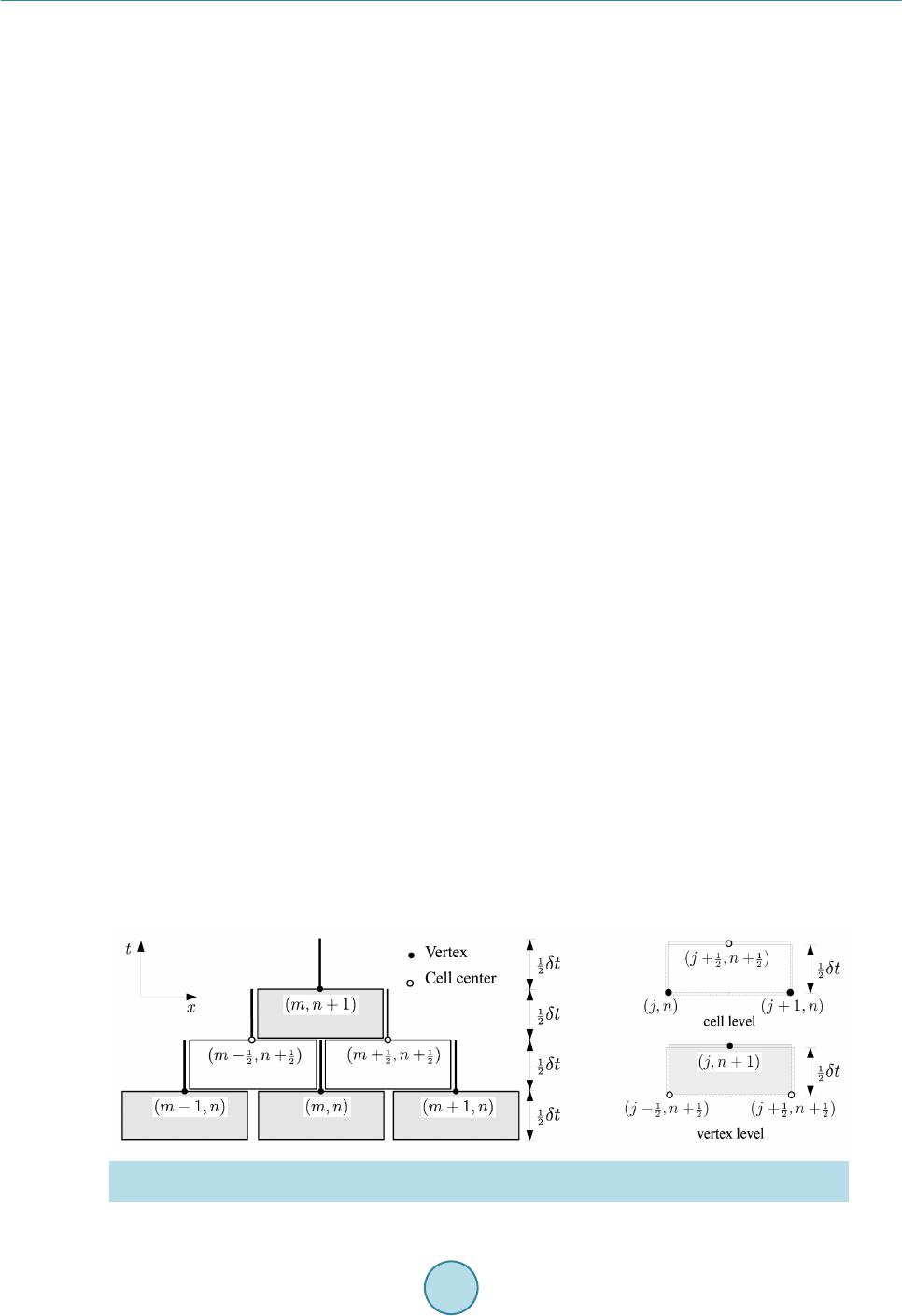

S. Z. Tu
56
unique inter face fluxes in solvers based on the finite volume method, discontinuous Galerkin method and some
other methods. Numerical methods based on Riemann solvers have achieved tremendous success in solving
hyperbolic systems, e.g., compressible Euler equations, where the eigenstructure of the system is clearly known,
in the past several decades. However, when physical processes get more complicated, for example, magnetohy-
drodynamics (MHD), the success of Riemann-solvers is far from satisfactory. For example, the Roe scheme [1]
has been modified to solve the MHD system. Roe’s scheme requires eigen-decomposition and becomes very
complicated in MHD equations. In addition, the Roe averages of quantitie s are not clearly defined in MHD system.
Moreover, due to the complexity and non-strict hyperbolicity of the MHD system, the validity of the eigen-
systems of the MHD system is not unanimously agreed upon among researchers. Therefore, Riemann-solver
free approaches are highly desirable to avoid the uncertainties caused by imperfect Riemann solvers.
In recent years, the author has been developing a Riemann-solver -free high order spacetime method for ar-
bitrary conservation laws [2]-[12]. The method is inspired by the spacetime Conservation Element/Solution
Element (CE/SE) [13] method and t he di s continuous Galerkin (DG) [14] method . The method integra t es the best
features of the two methods, i.e. the Riemann-solver-free feature of the CE/SE method and the high-order ac-
curacy of the DG method. The core idea of the method is to construct a staggered spacetime mesh through
alternate cell-centered CEs and vertex-centered CEs (cf. Figure 1 (right)) within each time step. Note that CEs
at the vertex level are defined via the dual mesh obtained by connecting the surrounding cell centers and face
centers. The difference between SEs and CEs is that the SE includes the volumeless vertical spike. Inside each
SE (cf. Figure 1 (left)), the solution is approximated using high-order spacetime DG basis polynomials. The
spacetime flux conservation is enforced inside each CE using the DG discretization. The unknowns are stored at
both vertices and cell centroids of the spatial mesh. However, the solutions at vertices and cell centroids are
updated at different time levels within each time step in an alternate fashion. Due to the alternate cell-vertex
solution upda ting strategy and its DG ingredient, the method has b e en termed a s the discontinuous Galerkin cell-
vertex scheme (DG-CVS) [4].
The method offers benefits to bo th the spacetime CE/SE method and the spacetime DG method. T he benefits
for the spacetime CE/SE method is two fold. First, DG-CVS increases the CE/SE method’s temporal and spatial
accuracies by emplo ying high-degree polynomial basis functions inside the SE. Second, DG-CVS pr esents uni-
versal defini tions of CEs and SEs for arbitrar y meshes. The CE a nd SE definition s in DG-CVS are independent
of the underlying spatial mesh and the same definitions can be easily extended from 1-D (cf. Figure 1) to
higher-dimensi ons (cf. Figure 2 and Figure 3) without any ambigui ty.
The benefits for the spacetime DG method are also two-fold . First, DG-CVS provides a Riemann-solver-free
approach for the DG methods. Second, DG-CVS does not need special treatment for the diffusion terms and thus
is conceptually simpler than e xist ing traditional DG methods for diffusion equations .
This paper summarizes the author’s work on DG-CVS in recent years. This paper is organized as follows.
Section 2 describes the current method in detail where the two ingredients of the method, spacetime DG method
and the alternate cell-vertex solution updating strategy, will be explained. In Section 3, many numerical ex-
amples are presented to demonstrate the accuracy of the method in solving various conservation laws including
scalar advection equations, compressible Euler equations, shallow water equations and MHD equations. Finally,
conclusion s will be summariz e d in Section 4.
Figure 1. Solution elements (SEs) and conservation elements (CEs) in the
xt−
domain. Left: solution
elements and right: conservation elements.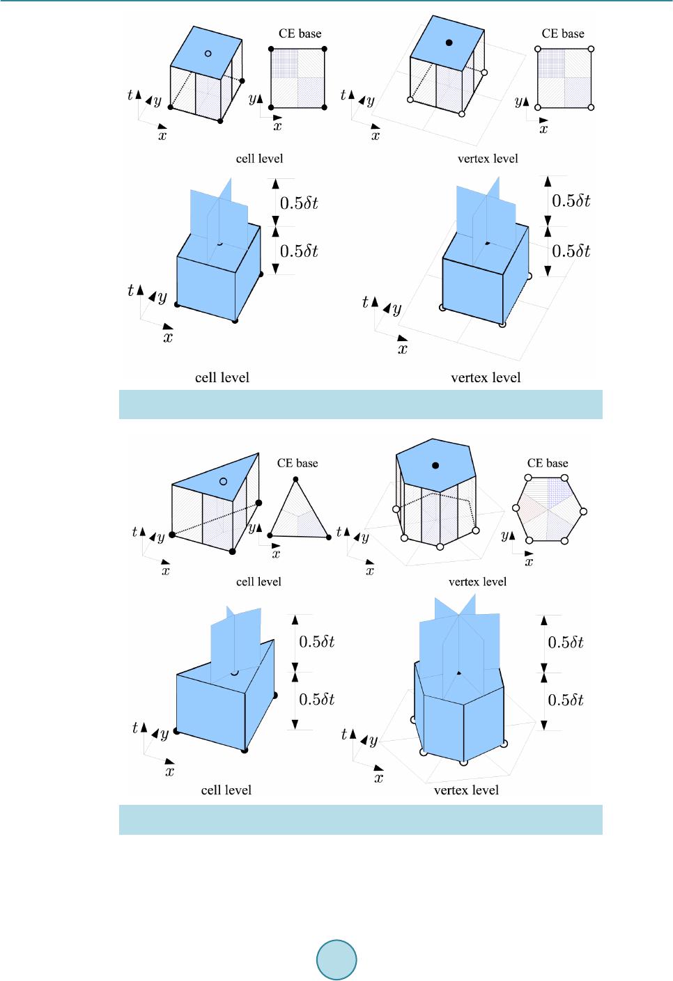

S. Z. Tu
57
Figure 2 . Conservation elements (CEs) and solution elements (SEs) for the quadrilateral mesh.
Top: CEs; bottom: SEs.
Figure 3. Conservation elements (CEs) and solution elements (SEs) for the triangular mesh.
Top: CEs; bottom: SEs.
2. Riemann-Solver Free Spacetime DG Method
To illustrate the Riemann-solver free discontinuous Galerkin (DG) formulation, we consider the following

S. Z. Tu
58
gener al one-dimensional time depe nde nt p a rtial differential e quation system
( )
,xt
tx
∂∂
+=
∂∂
ufr
(1)
that is used to describe many physical processes. Here,
u
is the solution vector containing the physical quan-
tities to be determined.
f
is the spatial flux vector. Without loss of generality, a source term
r
is also in-
cluded in Equation (1). Note that
f
may contain both advective and diffusive fluxes. Both
f
and
r
can be
functions of
u
or
∇u
or both. Appropriate initial and boundary conditions must also be provided to solve
Equation (1).
2.1. Spacetime Discontinuous Galerkin Formulation
Following the idea of the DG method, an approximate solution
h
u
is sought within each spacetime solution
element (SE), denoted as
K
. When restricted to the SE,
h
u
belongs to the finite dimensional space
( )
K
.
Assume all the components of the conservative variables inside each SE are approximated by polynomials of the
same degree, i.e.
( )()
1
,,
N
hjj
j
xt xt φ
=
=
∑
us
(2)
where
( ) { }
1
,
N
jj
xt φ
=
are some type of spacetime polynomial basis functions defined within the solution element,
{ }
1
N
jj
s
=
are the unknowns to be determined and N is the number of basis functions depending on the degree
of the polynomial function. Using such spacetime DG solution space, the solution approximation can be ar-
bitrarily high order accurate in both space and time.
Follow ing the G alerk in orth ogonality prin ci pl e, mult i ply (1) w ith each of the ba sis functi ons
i
φ
( )
1, 2,,iN=
and integrate over a spacetime CE to obtain the following weak form
d0, 1,2,,
K
hh
h
i
iN
tx
φ
Ω
 ∂∂
+ −Ω==

∂∂

∫uf
r
(3)
where
K
Ω
is the spacetime conservation element (CE) associated with the solution element K. Note that the
conservatio n element is identi cal to the solution ele ment except for the volumeless vertic al spike in the solu tion
element as shown in Figure 1. The spacetime flux conservation in weak form as in (3) is for each individual
spacetime conservation element. Therefore, the current method can be considered as a spacetime discontinuous
Galerkin method.
Integrating (3) by parts results in
dd
h hhh
ii
ii
K
tx
φφ
φφ
ΩΓ
∂∂

++Ω=⋅ Γ

∂∂

∫∫
uf rHn
(4)
where
( )
,
h hh
=H fu
(5)
is the spacetime flux tensor and
( )
,
xt
nn=n
is the outward unit normal of the CE boundary, i.e.
K
Γ = ∂Ω
, o f
the spacetime conservation element (CE) under consideration. Note that the partial integration is also performed
on the t ime -dependent term, which is a salient difference between spacetime DG methods and semi-discrete DG
met hods. As can b e seen, the formulation in (4) contains bot h the vo lume integral and the s urfac e inte gral.
2.2. Cell-Vertex Solution Updating Strategy
The current method inherits the core idea of the CE/SE method using a staggered spacetime mesh to enforce the
spacetime flux conservation. However, the construction of the staggered spacetime slabs in the current method
deviates from the CE/SE method. In the current method, unknowns are stored at both vertices and cell centroids
of the spatial mesh, and the solutions at vertices and cell centroids are updated at different time levels within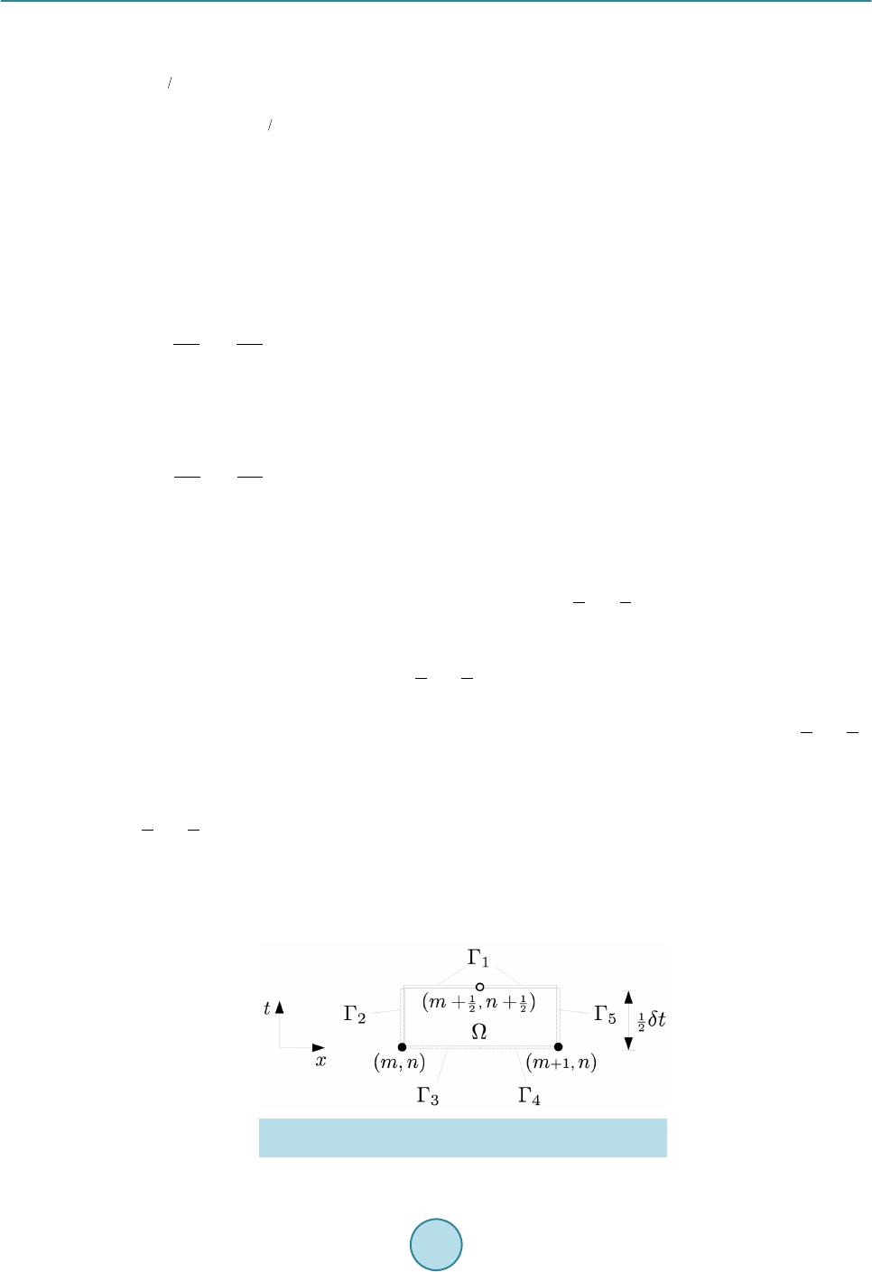

S. Z. Tu
59
each time step. At the beginning of each physical time step, the solution is a ssumed known at the cell centroids
of the mesh, either given as the initial condition or obtained from the previous time step. Inside each new time
step, the solution is updated in two successive steps. The first step updates the solution at vertices at the half-
time level
( )
12n
t
+
based on the known cell-centroid solutions at the previous time level
( )
n
t. The second step
updates the solution at cell centroids at the new time level
( )
1n
t
+
based on the known vertex solutions at the
pre vio us ha lf -time level
( )
12n
t
+
. The same pro cess is repeated for new time steps.
The solution updating at the cell level or the vertex level is based on the key equation (4). To evaluate the
integrals in (4), first divide the c onservation ele ment into the follo wing portions:
• The interior volume
K
Ω
where the solution is associated with the spacetime node at the new time level.
• The top surface
top
Γ
where the solution is also associated with the spacetime node at the new time level.
• The side surfaces
side
Γ
where the solution is associated with the spacetime node at the previous time level.
• The bottom surfaces
bott
Γ
where the solution is also associated with the spacetime node at the previous
time level.
Correspondingly, Equation (4) can be rearranged to yield
topside bott
dddd, 1,2,,
K
h hhhhh
ii
iiii
iN
tx
φφ
φφφ φ
Ω ΓΓΓ
∂∂

++Ω−⋅Γ=⋅Γ+⋅Γ =

∂∂

∫ ∫∫∫
uf rHnHnHn
(6)
where the left ha nd side contains the u nkno wns and the ri ght ha nd side contains the known information.
Since the top and the bottom surface of the CE are horizontal, which leads to
hh
⋅= Hnu
on the t o p fac e a nd
hh
⋅=−Hn u
on the bottom face, Equation (6) c a n be simplified to
top sidebott
dddd, 1,2,,
K
h hhhhh
ii
i iii
iN
tx
φφ
φ φφφ
ΩΓΓ Γ
∂∂

++Ω−Γ=⋅ Γ−Γ=

∂∂

∫∫∫ ∫
uf ruHnu
(7)
Equation (7) is a nonlinear equation system for each spacetime node which can be solved by the Newton-
Raphson iterative method.
To further illustrate the idea of enforcing the spacetime flux conservation, consider the conservation element
shown in Figure 4. Suppose the solution at the spacetime node
11
,
22
mn

++


is to be determined. Here,
m
and
n
represents the spatial and the temporal locations of the spacetime node, respectively. The boundaries of
the CE associated with the spacetime node
11
,
22
mn

++


is divided into five sections
1
Γ
,
2
Γ
,
3
Γ
,
4
Γ
and
5
Γ
, as s hown in Figure 4. Among t hese sect ions,
1
Γ
belongs to the SE associated with node
11
,
22
mn

++


where the solution is to be determined,
2
Γ
and
3
Γ
the SE associated with node
( )
,mn
and
4
Γ
and
5
Γ
the
SE associated with node
( )
1,mn+
. The interior volume of the conservation element is also associated with
node
11
,
22
mn

++


where the sol ution is to be found.
Due to the cell-vertex solution updati ng strategy and its D G i ngredi ent, the current method has b een termed as
the DG-CVS met hod [4].
Conventional DG methods use some type of Riemann solvers to provide numerical fluxes across element
Figure 4 . Illustrati on of spacetime flux con servation on a 1-D
cell-level CE.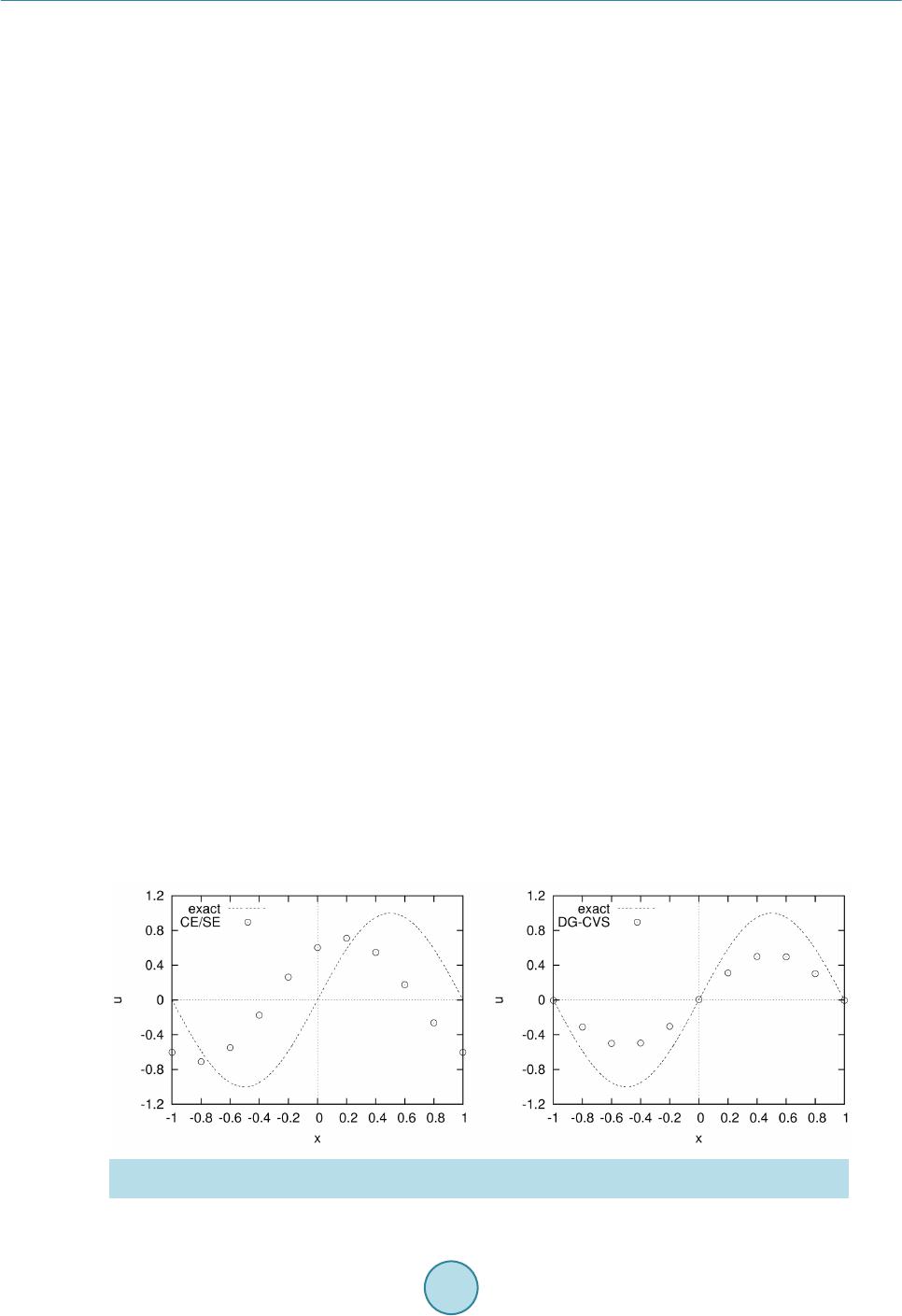

S. Z. Tu
60
interfaces. Thanks to the above explained staggered space-time for mulation, ther e is no “left” a nd “right” states
for the solution at the spacetime interface. Instead, the solution available to evaluate the flux is continuous
across the interface. Therefore, no (ap p r o ximate) Riemann solvers are needed to provide a unique numerical flux.
The Riemann-solve r-free feature is highly desirable for systems where the eigenstructure of the underlying
system is not readily known and for the purpose of avoiding some pathological behaviors (e.g., carbuncle
problem) associated with some Riemann solvers.
Note that in the CE/SE met hod [1 3], the time derivative of the solution is obtained from the spatial derivative
of t he so lut io n usi ng t he o ri gin al go ver ni ng e q uatio n. B y c on tr ast, i n t he c urr ent me tho d, t he t ime d er ivat ive of the
solution is treated as an independent unknown and handled in the same way as that for the spatial derivative of the
solution. Therefore, even for the same second-ord er ver sio n, the c urr ent me thod devi ates fro m the C E/SE met hod.
Figure 5 compares the solutions obtained from the CE/SE method and the current method for the sinusoidal wave
advection problem. It can be seen that the current method exhibits invisible phase error after 100 periods, which is
an outstanding feature in contrast to the C E/SE solution where sign if icant phas e error can be observ ed.
2.3. Quadrature-Free Implementation
If the underlying spatial mesh is unstructured (cf. Figure 5), the vertex-level CEs are general polygonal
cylinders containing general polygonal bases where the Gaussian quadrature rule cannot be directly applied.
Therefor e, it is de sired t hat t he volume integr al in Equation (7) is evaluated using a quadrature-free approach. In
addition, quadrature-free approaches help to significantly improve the efficiency of the method.
To allow the quadrature-free implementation, the flux and source vectors must be expanded in terms of the
basis polynomials similar to those used to expand the conservative variables, namely, for two-dimensional cases
11 1
, , and .
NN N
hh h
jj jjjj
jj j
φφ φ
= ==
= ==
∑∑ ∑
fg r
fsgs rs
 
(8)
where
N

is the number of basis polynomials of one degree higher than those to expand the conservative
variables as in Equation (2). The requirement of using basis polynomials of degree
1p+
for flux and source
term expansions is necessary to ensure the accuracy of the scheme.
The method based on the Cauchy-Kovalewski (CK) procedure [15] [16] is especially suitable for this purpose.
In the current method, the conservative variables are expanded using the Taylor polynomials. With the Taylor
polynomials, the spatial and temporal derivatives of the solution are explicitly available. Using the CK proce-
dure, the spacetime derivatives of the flux vectors can be obtained using the spacetime derivatives of the con-
servative variables.
With Taylor polynomials, the integrand of the volume integral has the following general form for two-
dimensional cases
( )
,,
l mn
q xytxyt=∆∆ ∆
(9)
which results from the products between Taylor polynomials. In (9),
, lm
and
n
are integer exponents. The
Figure 5. Comparison of the solutions of sinusoidal wave advection after 100 periods. Left: CE/SE. right:
current method (second-order version).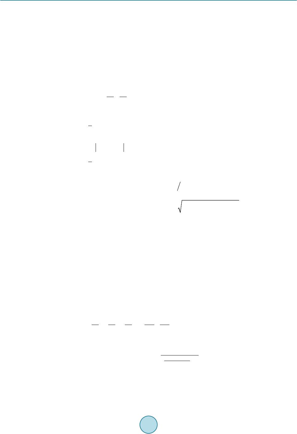

S. Z. Tu
61
idea is to use the divergence theorem explained in [17] to reduce the volume integral to surface integrals and
further to line integrals. The detailed procedure has been described in [4] and will not be repeated here.
3. Numerical Examples
In this section, various numerical cases are presented to demonstrate that current Riemann-solver free DG
method is able to solve many different types of conservation laws without using any Riemann-solvers.
3.1. Scalar Equation s
3.1.1. Linear Scalar Advection Equation
We first consider the following linear scalar advection equation:
0, 11
uu x
tx
∂∂
+=−≤ ≤
∂∂
(10)
with the initial co nd ition given as follows [18]:
( )
() ()() ( )
( )
() ()()
( )
1, ,, ,4, ,,0.80.6;
6
1,0.4 0.2;
1 100.100.2;
,0
1, ,, ,4,,,0.40.6;
6
0, otherwise.
Gx bGx bGxbx
x
xx
ux
Ex aEx aEx ax
βδ βδβ
αδ αδα
−+++−≤ ≤−

−≤ ≤−

− −≤≤
=

− ++ +≤≤



(11)
where
0.5a=
,
0.7b= −
,
0.005 δ =
,
10 α =
and
( )
2
log2 36 βδ =
.
G
and
E
are Gaussian and ellip-
tical function, r e spectively, w here
( )
( )
()( )
( )
2
2
2
,,eand,,max 1,0
xb
Gxb Exaxa
β
β αα
−−
== −−
It is clear that this problem is about the advection of mixed Gaussian, square, triangle and elliptical waves.
Periodic boundary conditions are assumed at the ends of the domain.
The computational domain is discretized by 200 evenly spaced cells which is a pretty coarse mesh for this
case. The time step used in all simulations is
0.0025 t δ =
corresponding to the Courant number
0.25 σ =
. To
resolve discontinuities, the limiting procedure described in [3] is used. Figure 6 shows the limited solutions at
8.0t=
using
1p
(second order) and
3p
(fourth order) basis polynomials, respectively. As can be seen, both
the discontin uities and s mooth region s are bette r captured with higher
p
. With increasing
p
, the transition of
discontinuities is steeper. The second order run is not able to resolve the Gaussian wave which is steep and
smooth. Another feature of the solution which is worthy of mentioning is that the wave profiles are symmetric,
which indicates the phase error of the current method is very small.
3.1.2. Burgers Equation
Here, the following 2-D visc ous Burge rs equation is solved.
22
22
0, 0, 25
uuu uu
u uxy
txy xy
ν

∂∂∂ ∂∂
++−+ =≤≤

∂∂∂ ∂∂

(12)
with the analytic al solution given as
( )
exact 2
2
,,
e1
cc
xx yyt
u xyt
ν
− +− −
=
+
where
( ) ()
, 0,0
cc
xy =
is a constant loca tion.
The 1-D version of this case was presented in [19]. This case is constructed such that the original wave is
propagated without chan ging shape u nder t he effect o f both nonlinear advection and linear diffusion. The initial

S. Z. Tu
62
Figure 6 . Linear advecti on of mixed waves. Li mited solu tion at
8.0t=
. The computational domain consists
of 200 uniform elements. Thick solid line: exact solution; circles and thin colorful solid lines: current
numerical solutions; and stars: oscillation indicators.
solution at
0t=
and the boundary conditions on all four boundaries are provided by the analytical solution.
Therefore the boundary conditions are time dependent.
In this test, a medium wave corresponding to
1=/ νδ x
is simulated using the present method. Figure 7 plots
the
1p
solution along the diagonal line
0xy−=
together with the exact solution. The
3p
solution is not
shown since no much visual difference can be seen between the
3p
soluti on and the
1p
soluti on. As can b e
seen, the wave has been captured accurately in terms of both location and magnitude. Figure 7 also compares
the computed solution gradients (
x
u
or
y
u
) with the exact solution. As can be seen, the
3p
solution is
superior to the
1p
solution in resolving the local sharp extremum of the solution gradient. This case demonstrate
that the current method is able to solve diffusion problems without any special tricks for diffusion terms as
required by many other DG methods. Note that the treat ment of diffusion terms in traditional semi-discrete DG
methods are non-trivial because of the so-called “variational cri me”. More test cases on diffusion problems have
been presented in [7].
3.1.3. Level Set Equation
The level set method introduced by Osher and Sethian [20] has been widely used to solve interface problems
emergi ng in ap plicatio ns such a s the two-pha se fluid d ynamic s, image se gmentat ion, co mputer vis ion and co m-
putational geometry etc. The biggest advantages of the level set method is that it naturall y allo ws the interface to
have topological changes due to the interface breaking and merging.
In the level set method, the interface is represented by the zero level set
( )() { }
,0tt ψ = =xx
of a level set
function
( )
,t ψ x
.
ψ
is often taken to be the signed distance function to the interface. The level set equation
can be expressed as
0
t
ψψ + ⋅∇=v
(13)
where
( )
,uv=v
is the velocity field which evolves the interface. Equation (13) can be rewritten in conser-
vative form
()
t
v ψ ψψ +∇⋅= ∇⋅v
(14)
Here, the DG-CVS method is used to solve Equation (14). In the two examples presented here, the com-
putational domain size is
[ ][ ]
0,1 0,1×
. The interface is represented by the zero level set of the signed distance
field. Since the interface evolution often occurs within a narrow band, the initial signed distance field is nar-
rowed by the following
, if;
, if;
, if.
ψ
ψψ ψ
ψ
− <−


=−≤ ≤

>




where

is chosen to be 0.1.

S. Z. Tu
63
Figure 7. Solution of 2-D viscous Burgers equation along the diagonal line
0xy−=
at
20T=
. Left:
u
, middle:
1p
x
u
and
y
u
, and right:
3p
x
u
and
y
u
.
The first well known example is the rigid rotation of the Zalesak disk [21]. The initial interface is a circle
centered at
( )
0.5,0.75
with a notch of width and depth 0.05 and 0.25, respectively. The velocity field is
( )
2π0.5uy= −
and
( )
2π0.5vx=−−
. The initial level set function is initialized as the signed distance to the
disk (Figure 8). The computational mesh contain s
50 50×
rectangular cells. The time step in the simulatio n is
0.00125t δ =
. 800 time steps were finish one revolution. Figure 9 shows the fo urth orde r
( )
3p
solution. Com-
pared to the exact solution, the smearing is very small which indicates the small numerical dissipation of this
high orde r scheme.
Another example is to simulate the deformation of a circular bubble of radius 015 centered at
( )
0.5,0.75
.
The circle is deformed due to the following velocity field [22]:
()()()( )( )( )
22
sin 2πsin πcosπ, and sin2πsin πcos πuyx tTvxy tT=−=
(15)
which are obtained from
( )
,yx−∂Ψ ∂∂Ψ ∂
where
Ψ
is the follo wi ng str e am function
( )( )
22
1sin πsin π
πxyΨ=
proposed in [22]. The time dependent term in (15) was proposed in [23] to contro l the magni tude a nd direction
of the velocity. At
2tT =
, the velocity starts to reverse direction and at time
tT=
, the original circle is ex-
pected to be restored.
The velocity field given b y (15) represents a vortex which stretch the circular fluid body into a thin filament
toward the vortex center. The simulation is performed on a relatively coarse
40 40×
mesh. Here
4T=
.
Figure 10 shows the fourth order
( )
3 p
evolution of the signed distance field and the zero level set at various
times. At
0.5 2tT==
, the bubble starts to restore its shape. At
4.0t=
, the bubble recovers its original cir-
cular shape. The comparison with the exact solution shows the accuracy of the current method. Note that
reinitialization is not needed with the current hig h o rder method in this case.
3.2. Compressible Euler Equation s
The two-dimensional co mpressible Euler equations can be wr itte n in the following vector form:
0
txy
∂∂∂
++=
∂∂∂
ufg
(16)
where
2
2
, , and
uv
uupuv
vvuv p
E HuHv
ρρ ρ
ρρ ρ
ρρ ρ
ρρ ρ
 
 
+
 
= ==
 
+
 
 
uf g
(17)
are the conservative state vector, flux vectors in
x
-and
y
-directions, resp ective ly. In (17 ),
ρ
,
u
,
v
,
p
,
E
,
and
H
are density,
x
- and
y
-components of the velocity, pressure and the total energy, and the total enthalpy,
respectively. Here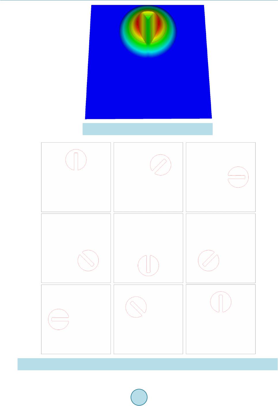

S. Z. Tu
64
Figure 8. Zalesak disk. Initial level set is the signed distance
to the disk.
Figure 9. Rotation of Zalesak disk. The locations of the disk at several instants within one revolution. The image order is
from left to right and from top to bottom.

S. Z. Tu
65
(a) (b) (c)
(d) (e) (f)
(g) (h) (i)
Figure 1 0.
3p
solution of the shearing of a circular bubble by a vortex on a
40 40×
mesh.
4T=
. (a) t = 0.0; (b) t = 0.5;
(c) t = 1.0; (d) t = 1.5; (e) t = 2.0 ; (f) t = 2.5; (g) t = 3.0; (h) t = 3.5; (i) t = 4.0.
( )
1ep γρ = −
()
22
1
e2 E uv=++
( )
22
1
e2
p
HEu v γ
ρ
=+=+ +
where
e
is the specific internal energy and
γ
is the ratio of sp e c ific heats.
This first Euler equation case is the classic Sod’s shocktube problem. The initial conditions are a high-
pressure region on the left and a lo w-pressure region on the right separated b y a diaphragm located at
0.5x=
.
At time
0t=
, the diaphragm is broken, a shock wave will propagate to the right and an expansion wave pro-
pagate to the left. There is a contact discontinuity in between across which the density and entropy are dis-
continuous while the pressure and velocity are continuous. The spatial domain is discretized into 100 equally
spaced eleme n t s . Figure 11 shows the comparison of
1p
numerical solution with exact solution at time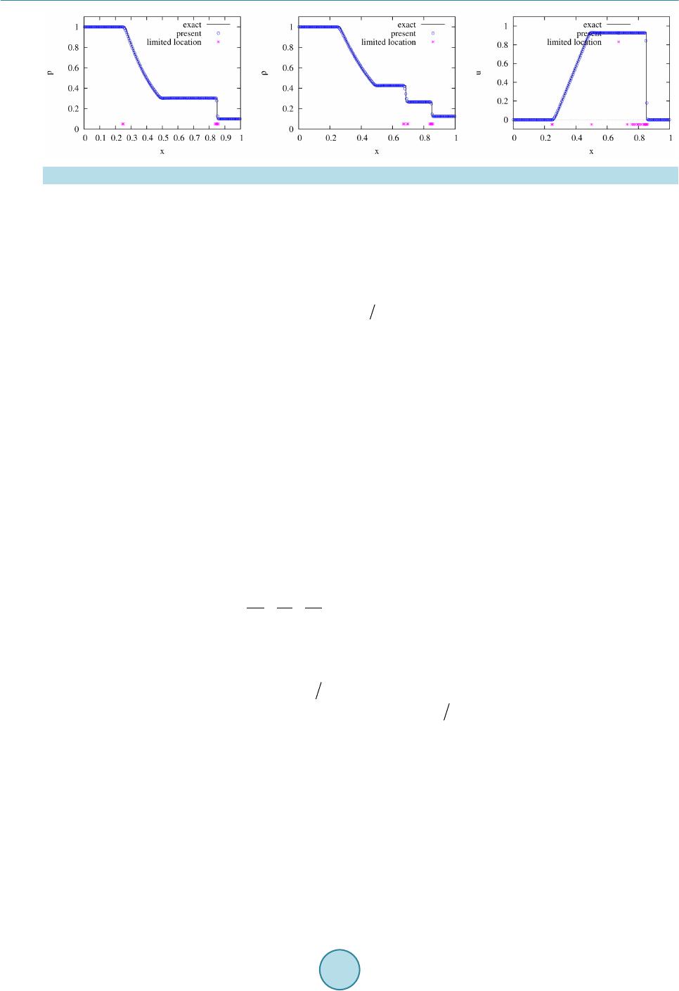

S. Z. Tu
66
Figure 1 1.
1p
s ol utions of Sod’s shocktube problem. Left: pressure, middle: density, and right: velocity.
0.2t=
. The good agreement in both wave location and sharpness demonstrates the accuracy of curren
Riemann-solver free method.
The second case is a supersonic flow with
3=M
flo wing through a channel o f l ength 3 a nd hei ght 1. A step
of height 0.2 stands at location 0.6 downstre am of the inlet. The step acts as an ob stacle to the sup ersonic inflow.
A transient detached shock wave will be formed and hit the top wall. The shock wave will reflect from the top
wall a nd fur ther h it the bott om wall a nd r eflec t agai n. The flo w expand s rap idly at t he si ngula rity c orner . In t he
present simulation, a rectangular mesh of
1 40xy δδ = =
is used. The linear basis polynomials
( )
1p
is
employed in this test. Figure 12 shows the densit y field at
4.0 t=
. As c an b e see n, t he main fea ture s inc lud ing
the detached bow shock, the Mach stem below the top wall, slip line, reflected shock waves are well captured.
Here, no any type of boundary conditions is applied at the singularity corner and no numerical difficulty was en-
countered. No expansion shocks are seen around the corner. In addition, the present method does not exhibit t he
so-called carbuncle problem in the subsonic region behind the bow shock.
To illustrate the mesh flexibility of the current method, a simulation about a nearly incompressible subsonic
flow with Mach number
0.1M=
passing around a circular cylinder with radius
0.5 R=
on an overset
Cartesian/quadrilateral mesh is presented. Figure 13 s hows the nea r-body pressure field at the steady state with
the background overset mesh also displayed. Indeed, the current method works for arbitrarily unstructured
meshes.
3.3. Shallow Water Equations
The shallow water equations (SWE) are widely used as the mathematical model to numerically simulate the dam
break, river inundation, failure of levees and tide of ocean in coastal and civil engineering. The frictionless
shallow water equation can be expressed in the following conservative form
( )
txy
∂∂∂
++=
∂∂∂
ufg
ru
(18)
in which the conservative vector , flux vectors and source vector are
22 0
22 0
0
, 2, , and
2
x
y
H HuHv
HuHugHHuvgHS
HvHuvHv gHgHS

 
 
==+= =

 
 
+
 
uf gr
respectively. Here, the total water depth
( )( )()
,,Ht td ζ = +x xx
where
( )
,t ζ x
is the free-surface elevation
and
( )
dx
is the still water depth.
u
and
v
are the
x
- and
y
-component of the depth-averaged velocity.
g
is the acceleration due to gravity.
0x
S
and
0y
S
are the bottom slopes in
x
- and
y
-directions, respec-
tively. If the bottom has zero slope, the source terms in Equation (18) would be absent.
The first shallow water case is a two-dimensional shocktube problem which is analogous to the shocktube
problem used to verify a compressible Euler solver. The computational domain is a
[ ][]
5,55,5− ×−
rectangular
region. At
0t=
, the lower left corner
[] []
5,0 5,0− ×−
of the domain is filled with water of height
4
3.0h=
,
and the rest of the domain is fi lled with water of height
10.03h=
. Symmetry conditions are assumed on the left
and the bottom boundaries of the domain. The domain is discretized into
99 99×
evenly distributed rectangular
cells. The simulation is run till
2.0t=
at which the shock is still within the domain. The solutions along the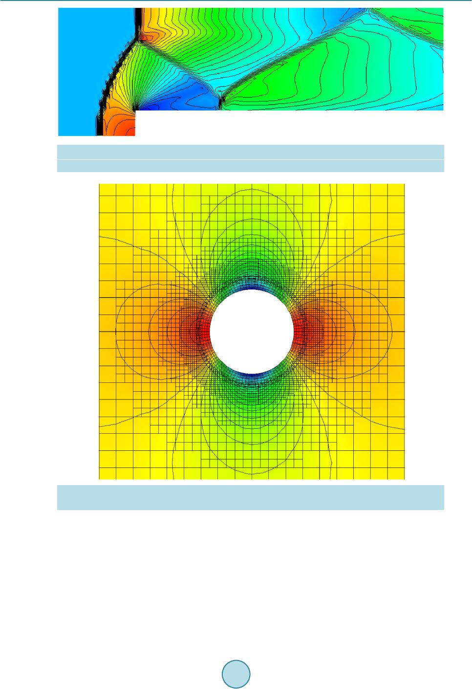

S. Z. Tu
67
Figure 12. Density field of a supersonic
( )
3M=
flow through a channel with a forward-facing step at
4.0t=
.
Figure 13. Steady pressure field of the inviscid flow
( )
0.1M=
passing around a circular cylinder. The
overset Car tesian and quadrilateral mesh is displayed at background.
symmetry boundaries are identical to those in the 1-D case. T herefore, the available analytical solutions [24] ca
be used to verif y the present numerical solution.
Figure 14 shows the
1p
solutions along the bottom symmetry boundary. The analytical solutions are also
shown for comparison purpose. As can be seen, the shock location and strength have been captured very well.
This is in contra st to the results reporte d in [25] s howing th at the leas t-square finite ele ment method is not able
to capture the strong shock in the rig ht loc a tion.
The second case is another classical benchmark problem widely used to verify shallow water equation solvers
[26]. Figure 15 (left) depicts the domain geometry. Initially, two reservoirs are separated by a lock gate which is
of 75 meters wide. The water levels are 10 meters and 5 meters, respectively. The reservoir on the left has higher

S. Z. Tu
68
Figure 1 4. Shallow water shocktube problem.
Figure 1 5. 2-D dam break problem. Left: geometry, right: carpet view of the water elevation at
7.2 s t=
.
water level. The resolution of the co mputational mesh is 2.5 meters. At
0t=
, the lock gate is opened. Figure
15 shows the carpet view of the water level at
7.2t=
seconds. The
1p
solution qualita tively compares well
with that in [26] where a Riemann-solve r-based method is used.
3.4. MHD Equat ion s
3.4.1.
33×
MHD Model Equations
The present Riemann-solve r-free method is first a pplie d to solve the following
33×
MHD model system in the
phase space which exactly preserves the MHD singularities [27]:
t xxx
+=u fdu
(19)
with
22 2
00
, 2, and 0
20
ucu v w
v uv
w uw
µ
ηχ
χη

++
 

 
= ==−

 
 

 

uf d
where the longitudinal viscosity
µ
and the magnetic resistivity
η
are the dissipative coefficients, and the
Hall coefficient
χ
is a dispersive coefficient. The above quantities are related to the MHD system via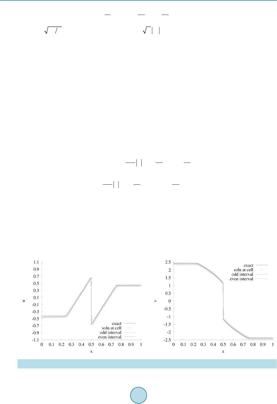

S. Z. Tu
69
2
1, , , and 1
yz
a xx
BB
a
uvw c
c BB
γ

= −===+


where
ap γρ =
is the acoustic wave speed,
ax
cB ρ =
is the Alfven wave speed,
p
is the pressure,
ρ
is the d ensity and
γ
is the ratio of specific heats. T he model system (19) generates three wave families which
are the Alfven wave, the slow and the fast MHD waves. This model system has been investigated by several
authors [27] [28] to provide insights to improve Godunov-typed numerical schemes for MHD equations.
The test case presented here is taken from Ref. [28] where conventional and modified Roe’s scheme were
used to solve the system. In this case,
3c=
and the computational domain
[ ]
0,1
is evenly divided into 150
cells. The dissipative term on the right hand side of (19) is assumed to be zero.
The initial disco ntin uity is an entro p y-violating shock defined as
( )
0.44,2.4,0
LR
=−=−uu
. The final time is
0.0376506024t=
. 150 time steps have been run to reach the final ti me. Figure 16 shows
u
vs.
x
and
v
vs.
x
solutions from the second order simulation along with the analytical solutions. The agreement is very well
and the overshoots/ undershoots around the disconti nuity regi on have been suppresse d using a slo pe limiter .
3.4.2. Ideal Compressible MHD Equ ations
The ideal compressible MHD equations combines the Euler equations of gas dynamics with Maxwell equations
of electromagnetics for problems in which viscous, resistive and relativistic effects can be neglected. The ideal
MHD equations contain a set of nonlinear hyper bolic equa tions as shown in the following conservati ve form:
()
0
t
ρρ ∂ +∇⋅=v
(20)
( )
2
00 0
111
2
t
p ρρ µµµ


∂+∇⋅+ +−=−∇⋅





vvvBIBBB B
(21)
( )( )( )
2
00 0
11 1
2
t
E Ep ρρµµµ


∂+∇⋅+ +−⋅=−⋅∇⋅





B vBvBvBB
(22)
( )
t
∂+∇⋅−=− ∇⋅BvB BvvB
(23)
Here,
ρ
,
v
,
E
,
P
,
0
µ
and
( )
T
,,
xyz
BBB =B
represent the mass density, the velocity vector, the total
energy, the hydrodynamic pressure, permeability of vacuum and the magnetic field. In addition to satisfying the
induction equation (Equation (23) above), the magnetic field is also divergence free, i.e.
0∇⋅ =B
which can
be considered as an extra constraint. Note that in Equations (20)-(23), the so-called Powell approach [29] is
followed to deal with
0∇⋅ =B
by adding source terms proportional to
∇⋅B
to the equation s.
The first MHD case presented here is known as the Brio-Wu case [30] which is a one-dimensional MHD
Figure 1 6. Solutions of the Myong case.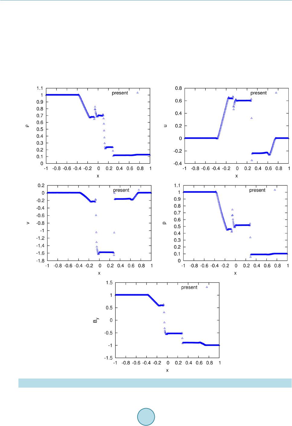
( )
0.44,2.4,0
LR
=−=−uu
at
0.0376506024t=
.

S. Z. Tu
70
Riemann problem on the computational domain
[ ]
1,1−
. The initial states are given in the form of primitive
variables
T
,,, , ,,
yz
uvwpB B ρ

= q
separated at
0x=
() ()
TT
1.000,0,0,0,1.0,1.0,0.0, and 0.125,0,0,0,0.1,1.0,0.0
LR
== −qq
with
0.75
x
B=
and
2 γ =
.
Figure 17 shows the simulated solution at
0.2 t=
. As can be seen, the complex MHD waves including the
compound wave, the shock wave, contact discontinuity and rarefaction waves can be captured by the present
Riemann-solver free method. However, the unlimited solutions exhibit some non-physical overshoots and
undershoots near discontinuities.
Figure 1 7. Solutions of the Brio-Wu case.
0.75
x
B=
.
0.2t=
.

S. Z. Tu
71
Finally, preliminary results of a 2-D MHD vortex advection problem are presented. The case is about a vortex
advected with the magnetic field diagonally in a square
[ ][ ]
5,55,5− ×−
domain. Periodic boundary conditions
are assumed. The computational domain is discretized by a
32 32×
rectangular mesh. The solution is initialized
as follows [31]:
( )
( )
()
( )
( )
( )
()
2
2
2
2
2
0.5 1
0.5 1
12
2
0.5 1
0.5 1
1.0,
1
1.0 e,
2π
1
1.0 e,
2π
0.0,
1
1.0 e,
8π
1e,
2π
1e,
2π
0.0.
r
r
r
r
x
r
y
z
uy
vx
w
pr
By
Bx
B
ρ
−
−
−
−
−
=
=+−
= +
=
=+−
= −
=
=
where
222
rxy= +
.
Figure 18 sho ws the magnetic field and velocity magnitud e field at
0.0 T=
and
10.0T=
. It can seen that
the solution fields have been preserved well after one period’s advection.
4. Conclusions
This paper summarizes a Riemann-solver free spacetime discontinuous Galerkin method for general hyperbolic
conservation laws. Numerical examples demonstrate that the method is able to accurately solve various con-
servation laws including the scalar advection equations, compressible Euler equations, shallow water equations
and magnetohydrodynamics equations without using any Riemann solvers. To summarize, the method has the
following feature s:
• Based on space-time formulation. Therefore, the current method automatically satisfies the Geometric
Conservation Law (GCL) for moving mesh problems [10] without special care as needed by ALE-based
methods.
• High-order accuracy in both space and time for smooth problems. Space and time are handled in a unified
way based on space-time flux conservation and high-order space-time discontinuous basis functions. This is in
contrast to se mi-discrete methods where the temporal order of accuracy is limited by the order of Backward Dif-
ference Formula (BDF) or the multi-step Runge-Kutta method.
• Riemann-solve r free. DG-CVS does not need (approximate) Riemann solvers to provide numerical fluxes as
needed in finite volume or traditional DG methods. The Riemann-so lver -free feature is highly desirable for
syste ms wher e the eige nstr uctur e of the underlying system is not readily known and for the purpose of avoiding
some patholog ic a l behaviors associa te d with Riema nn solvers.
• Reconstruction free. DG-CVS solves for the solution and its all spatial and temporal derivatives simul-
taneously at each spacetime node, thus eliminating the need of reconstruction.
• Suitable for arbitrary spatial meshes. T he CE and SE defi nitio ns in D G-CVS a re ind epe ndent o f the und er -
lying spatial mesh and the same definitions can be easily extended from 1-D to 2-D arbitrarily unstructured
meshes wit hout a ny ambiguity.
• Highly compact regardless of order of accuracy. Only infor matio n at the i mmediat e neighb orin g node s will
be needed to update the solution at the new time level. Compactness eases the parallelization of th e flow so lver.
• Also a ccurately solves time-dependent diffusion equations. In the cur rent metho d, the in clusio n of diffusion
terms is straightforward and simple in exactly the same way how advection terms are handled by simply in-
corporating the diffusi ve fl ux i nto the sp ac e-time flux. No extra reconstruction or recovery or ad hoc penalty a nd
coupling terms are needed to ensure the consistency of the variational form for diffusive terms.
The future work remains to further improve the efficiency of the method and the robustness of the method

S. Z. Tu
72
(a) Bx-field. Left t = 0.0 , right t = 10.0
(b) By-field. Left t = 0.0, right t = 10.0
(c) Velocity magnitude field. Left t = 0.0, rig ht t = 10.0
Figure 1 8. MHD vortex advection problem.
when high order polynomials are used for nonsmooth problems.
Acknowledgem ents
This work presented in this paper is supported by the U.S. Air Force Office of Scientific Research (AFOSR)
Computational Mathematics Program under the Award Numbers FA9550-08-1-0122, FA9550-10-1-0045 and

S. Z. Tu
73
FA9550-13-1-0092. The authors are also grateful to the School of Engineering and the Department of Computer
Engi neering at J ackson State University for thei r supp ort.
References
[1] Roe, P. (1981) Approxi mate Riemann Solvers, P arameter V ectors, and Differen ce Sche mes. Journal of Computational
Physics, 43, 357-372. http://dx.doi.org/10.1016/0021-9991(81)9 0128-5
[2] Tu, S. (2009) A High Order Space-Time Riemann-Solver-Free Method for Solving Compressible Euler Equations.
Proceedings of the 47th AIAA Aerospace Scien ces Meeting including the New Horizons Forum and Aerospace Exposi-
tion, Orlando, 5-8 January 2009, AIAA Paper 2009-1335. http://dx.doi.org/10.2514/6.2009-1335
[3] Tu, S. (2009) A Solution Limiting Procedure for an Arbitrarily High Order Space-Time Method. Proceedings of the
19th AIAA Computational Fl ui d D y nam i c s Confe r e nc e , San Antonio, 22-25 June 20 09, AIAA Paper 2009-3983.
[4] Tu, S., S kelton, G. and P ang, Q. (2011) A Co mpact high Order Space-Ti me Method for Conser vation La ws. Commu-
nications in Computational Physics, 9, 441-480.
[5] Tu, S. and Tian, Z. (2010) Preliminary Implementation of a High Order Space-Time Method on Overset Cartesian/
Quadrilateral Grids. Proceedings of the 48th AIAA Aerospace Sciences Meeting Including the New Horizons Forum
and Aerospace Exposition, Orlando, 4-7 January 2010, AIAA Paper 2010-0544.http://dx.doi.org/10.2514/6.2010-544
[6] Tu, S., Pang, Q. and Xiang, H. (2011) Wave Computation Using a High Order Space-Time Riemann S olver Free Me-
thod. Proceedings of the 17th AIAA/CEAS Aeroacoustics Conference, Portland, 5-8 June 2011, AIAA Paper 2011-
2846.
[7] Tu, S., Skelton, G. and P an g, Q. (2012) Extension of the High-Order Space-Time Discontinuous Galerkin Cell Vertex
Scheme to Solve Time Dependent Diffusion Equations. Communications in Computational Physics, 11, 1503-1524.
http://dx.doi.org/10.4208/cicp.050810.090611a
[8] Tu, S., P an g, Q. and Xiang, H. (2012) Solving the Shallow Water Equations Using the High Order Space-Time Dis-
continuous Galerkin Cell-Vert ex Scheme. Proceedings of the 50th AIAA A erospace Scien ce Meetings, Nashville, 9-12
January 2012, AIA A Paper 2012 -0307.
[9] Tu, S., Pang, Q. and Xiang, H. (2012) Solving the Level Set Equation Using the High Order Space-Time Disconti-
nuous Galerkin Cell-Vertex Sche me. Proceedings of the 50th AIAA Aerospace S cience Meetin gs, Nashville, 9-12 Jan-
uary 2012, AIAA Paper 2012-1233. http://dx.doi.org/10.2514/6.2012-1233
[10] Tu, S. and Pang, Q. (2012) Development of the High Order Space-Time Discontinuous Galerkin Cell Vertex Scheme
(DG-CVS) for Moving Mesh Problems. Proceedings of the 42nd AIAA Fluid Dynamics Conference, New Orleans, 25-
28 June 2012, AIA A Paper 2012 -2835. http://dx.doi.org/10.2514/6.2012-2835
[11] Tu, S., Pang, Q. and Myong, R. (2013) A Ri e man n -So lver Free S pace-Time Discontinuous Galerkin Method for Mag-
netohydrodynamics. Proceedings of the 44th AIAA Plasmadynamics and Lasers Conference, San Diego, 24-27 June
2013, AIAA Paper 2013-2755. http://dx.doi.org/10.2514/6.2013-2755
[12] Tu, S., Song, H., Ji, L. and Pa ng , Q. (2015) Furth er Development of a Riemann-Solver F ree Space-Time Discontinuous
Galerkin Method for Compressible Magnetohydrodynamics (MHD) Equations. Proceedings of the 53rd AIAA Aero-
space Sciences Meeting, Kiss immee, 5-9 January 2015, AIAA Paper 2015-0567.
[13] Chang, S.-C. and To, W. (1991) A New Numerical Framework for Solving Conservation Laws: The Method of
Space-Time Conservation Element and Solution Element. NASA T M 1991-104495.
[14] Cockburn, B. and Shu, C.-W. (2001) Runge-Kutta Discontinuous Galerkin Methods for Convection-Dominated Prob-
lems. Journal of Scientific Computing, 16, 173-261. http://dx.doi.org/10.1023/A:1012873910884
[15] Dyson, R. (2001) Technique for Very High Order Nonlinear Simulation and Validation. NASA/TM 2001-210985.
[16] Dumbser, M., Käserb, M., Titarevb, V.A. and Toro, E.F. (2007) Quadrature-Free Non-Oscillatory Finite Volume
Schemes on Unstructured Meshes for Nonlinear Hyperbolic Systems. Journal of Computational Physics, 226 , 2 04-243 .
http://dx.doi.org/10.1016/j.jcp.2007.04.004
[17] Dasgupta, G. (2003) Integ ra tion within Polyg onal Finite Eleme nts. J ournal of A e r os pac e Enginee r ing, 16, 9-18.
http://dx.doi.org/10.1061/(ASCE)0893-1321(2003)16:1(9)
[18] Jiang, G. and Shu, C.-W. (1996) Efficient Implementation of Weighted ENO Schemes. Journal of Computational Phy-
sics, 126, 202-228. http://dx.doi.org/10.1006/jcph.1996.0130
[19] Popescu, M., Shy y, W. and Garb ey, M. (2005) Finite Volume Treatment of Dispersion-Relation-Preserving and Opti-
mized Prefactored Compact Schemes for Wave Propagatio n. Journal of Computational Physics, 210, 705 -729.
http://dx.doi.org/10.1016/j.jcp.2005.05.011
[20] Osher, S. and Sethian, J.A. (1 988) Fronts Propagating with Curvature-Dependent Speed: Algorithms Based on Hamil-

S. Z. Tu
74
ton-Jacobi Formulations. Journal of Computational Physics, 79, 12-49.
http://dx.doi.org/10.1016/0021-9991(88)90002-2
[21] Zalesak, S. (1979) Fully Multidimensional Flux-Corrected Transport Algorithms for Fluids. Jo urnal o f Comput ational
Physics, 31, 335-362. http://dx.doi.org/10.1016/0021-9991(79)9 0051-2
[22] Bell, J.B., Colella, P. and Glaz, H.M. (1989) A Second-Order Projection Method for the Incompressible Navier-Stokes
Equations. J ournal of C om p ut at i o nal Phy s i c s , 85, 257-283. http://dx.doi.org/10.1016/0021-9991(89)90151-4
[23] Le Veque, R.J. (1996 ) High Resolution Conservative Algorithms for Advection in Incompressible Flow. SIAM Journal
on Numerical Analysis, 33, 627-665. http://dx.doi.org/10.1137/0733033
[24] Tan, W. (1992) Shallow Water Hydrodynamics: Mathematical Theory and Numerical Solution for a Two-Dimensional
System of Shallow Water Equations. Elsevier Oceanography Series, Water & Power Press, Beijing.
[25] Liang, S.-J. and Hsu, T.-W. (2009) Least-Squares Finite-Element Method for Shallow-Water Equations with Source
Terms. Acta Mechanica Sinica, 25, 597-610. http://dx.doi.org/10.1007/s10409-009-0250-x
[26] Cueto-Felgueroso, L., Colominas, I., Fe, J., Navarrina, F. and Casteleiro, M. (2005) High-Order Finite Volume
Schemes on Unstructured Grids Using Moving Least-Squares Reconstruction. Application to Shallow Water Dynamics.
International Journal for Numerical Methods in Engineering, 65, 295-331. http://dx.doi.org/10.1002/nme.1442
[27] Myong, R. and Roe, P. (1997) Shock Waves and Rarefaction Waves in Magnetohydrodynamics. Part 1. A Model Sys-
tem. Journal of Plasma Physics, 58, 485-519. http://dx.doi.org/10.1017/S002237789700593X
[28] Myong, R.S. and Roe, P.L. (1998) On Godunov-Type Schemes for Magnetohydrodynamics. Journal of Computational
Physics, 147, 545-567. http://dx.doi.org/10.1006/jcph.1998.6101
[29] Powell, K.G., Roe, P.L., Linde, T. J., Gombosi, T.I. and De Zeeuw, D.L. (1999) A Solution-Adaptive Upwind Scheme
for Ideal Magnetohydrodynamics. Journ al of Computational Physics, 154, 284-30 9.
http://dx.doi.org/10.1006/jcph.1999.6299
[30] Brio, M. and Wu, C.C. (1988) An Upwind Differencing Scheme for the Equations of Ideal Magnetohydrodynamics.
Journal of Computational Physics, 75, 400-422. http://dx.doi.org/10.1016/0021-9991(88) 90120-9
[31] Li, F. and Shu, C.-W. (2005) Locally Divergen ce-Free Discontinuous Galerkin Methods for MHD Equations. Journal
of Scientific Computing, 22-23, 413-442. http://dx.doi.org/10.1007/s10915-004 -4146-4