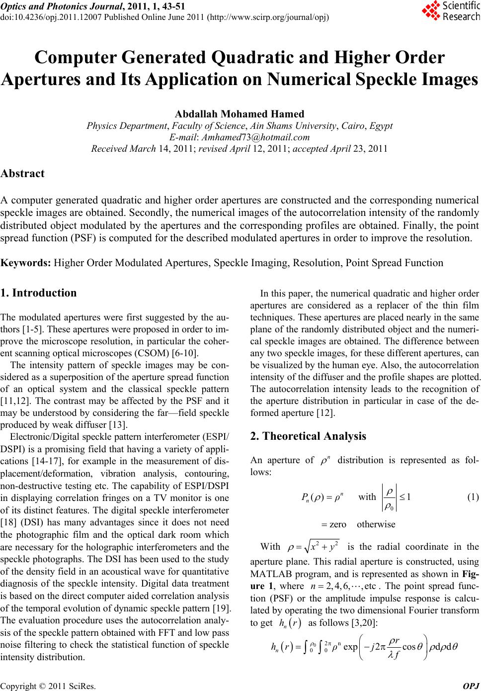Optics and Photonics Journal, 2011, 1, 43-51
doi:10.4236/opj.2011.12007 Published Online June 2011 (http://www.scirp.org/journal/opj)
Computer Generated Quadratic and Higher Order
Apertures and Its Application on Numerical Speckle Images
Abdallah Mohamed Hamed
Physics Department, Faculty of Science, Ain Shams University, Cairo, Egypt
Received March 14, 2011; revised April 12, 2011; accepted April 23, 2011
Abstract
A computer generated quadratic and higher order apertures are constructed and the corresponding numerical
speckle images are obtained. Secondly, the numerical images of the autocorrelation intensity of the randomly
distributed object modulated by the apertures and the corresponding profiles are obtained. Finally, the point
spread function (PSF) is computed for the described modulated apertures in order to improve the resolution.
Keywords: Higher Order Modulated Apertures, Speckle Imaging, Resolution, Point Spread Function
1. Introduction
The modulated apertures were first suggested by the au-
thors [1-5]. These apertures were proposed in order to im-
prove the microscope resolution, in particular the coher-
ent scanning optical microscopes (CSOM) [6-10].
The intensity pattern of speckle images may be con-
sidered as a superposition of the aperture spread function
of an optical system and the classical speckle pattern
[11,12]. The contrast may be affected by the PSF and it
may be understood by considering the far—field speckle
produced by weak diffuser [13].
Electronic/Digital speckle pattern interferometer (ESPI/
DSPI) is a promising field that having a variety of appli-
cations [14-17], for example in the measurement of dis-
placement/deformation, vibration analysis, contouring,
non-destructive testing etc. The capability of ESPI/DSPI
in displaying correlation fringes on a TV monitor is one
of its distinct features. The digital speckle interferometer
[18] (DSI) has many advantages since it does not need
the photographic film and the optical dark room which
are necessary for the holographic interferometers and the
speckle photographs. The DSI has been used to the study
of the density field in an acoustical wave for quantitative
diagnosis of the speckle intensity. Digital data treatment
is based on the direct computer aided correlation analysis
of the temporal evolution of dynamic speckle pattern [19].
The evaluation procedure uses the autocorrelation analy-
sis of the speckle pattern obtained with FFT and low pass
noise filtering to check the statistical function of speckle
intensity distribution.
In this paper, the numerical quadratic and higher order
apertures are considered as a replacer of the thin film
techniques. These apertures are placed nearly in the same
plane of the randomly distributed object and the numeri-
cal speckle images are obtained. The difference between
any two speckle images, for these different apertures, can
be visualized by the human eye. Also, the autocorrelation
intensity of the diffuser and the profile shapes are plotted.
The autocorrelation intensity leads to the recognition of
the aperture distribution in particular in case of the de-
formed aperture [12].
2. Theoretical Analysis
An aperture of n

distribution is represented as fol-
lows:
0
( )with1
n
n
Pρ



 (1)
zero otherwise

With 22
x
y   is the radial coordinate in the
aperture plane. This radial aperture is constructed, using
MATLAB program, and is represented as shown in Fig-
ure 1, where 2, 4, 6,, etcn

. The point spread func-
tion (PSF) or the amplitude impulse response is calcu-
lated by operating the two dimensional Fourier transform
to get


n
hr as follows [3,20]:

02n
00 exp2cosd d
n
r
hr ρjf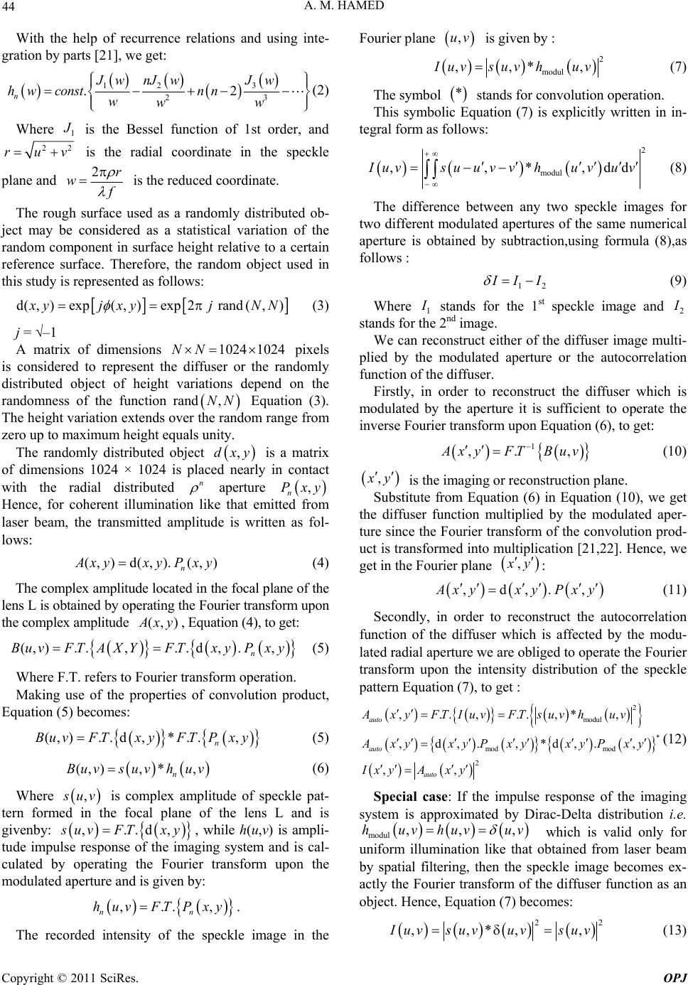











A. M. HAMED
44
With the help of recurrence relations and using nte-
gration by parts [21], we get:
i
   

12 3
23
.2
n
Jw nJwJw
wconstn n
ww






(2)
hw


Where 1
J
is the Bessel function of 1st order, and
22
ruv is the radial coordinate in the speck
pl
le
ane and 2r
w
f


urface used as a randomly distributed ob-
ject may bd as a statistical variation

 is the reduced coordinate.
The rough s
e considere of the
random component in surface height relative to a certain
reference surface. Therefore, the random object used in
this study is represented as follows:




d(,)exp(,)exp2rand( ,)
x
yjxy jNN   (3)
j = –1
A matrix of dimensions
is considered to represent tnd
dibject of heighton the
ra
1024 1024NN 
he diffuser or the ra
variations depend
rand

,NN Equati
pixels
omly
stributed o
ndomness of the function on (3).
The height variation extends over the random range from
zero up to maximum height equals unity.
The randomly distributed object

y is a matrix
of dimensions 1024 × 1024 is placed nearly in contact
with the radial distributed n

,dx

aperture


,Pxy
n
ence, for coherent illumination likmitted from
laser beam, the transmitted amplitude is written as fol-
lows:
(, )d(, ).(, )
n
He that e
A
xyxyP xy (4)
The complex amplitude located in the focal plane of the
lens L is obtained by operating the Fou
the complex amplitude
rier transform upon
(, )
A
xy , Equati
ourier
Making use of the properties of convolution pr
Equation (5) becomes:
on (4), to get:
   
(,)..,..d ,.,
n
BuvFTAXYFTx yPx y (5)
Where F.T. refers to F transform operation.
oduct,
   
(,)..d,* ..,
n
BuvFTx yFTPxy (5)



, *,
n
vhuv (, )Buvsu (6)
Where

,
s
uv

is complex amplitude of
tern formed in the focal plane of
givenby:
speckle pat-
the lens L and is
 
,..d,
s
uv 
lse resp
FTxy , wh
tu
aperture and is given b
ile h(u,v) is ampli-
de impuonse of the imaging system and is cal-
culated by operating the Fourier transform upon the
modulatedy:
 


,..,
nn
huv FTPxy.
The recorded intensity of the sp


,uv is given by :
 
eckle image in the
Fourier plane
2
modul
,,*,
I
uvsuvhuv (7)
The symbol


*
bolic Equation
stands for convolution operation.
This sym(7) is explicitly
tegral form as follows:
written in in-
 
2
modul
,,*,dd
I
uvsu uvvhuvuv



 
 (8)
The difference between any two speckle ima
two different modulated apertures of the same nu
aperture is obtained by subtraction,using formula (8),as
fo
ges for
merical
llows :
12
I
II


 (9)
Where 1
I
stands for the 1 speckle image and
st
2
I
stands fo2nd image.
We can reconstruct either of the diffuser image m
pl hen
upon Equation (6), to get:
r the
ulti-
ied by t modulated aperture or the autocorrelatio
function of the diffuser.
Firstly, in order to reconstruct the diffuser which is
modulated by the aperture it is sufficient to operate the
inverse Fourier transform



1
,. ,
A
xyFTBuv


 (10)


,
x
y

 is the imaging or reconstruction plane.
Substitute from Equation (6) in Equa
the diffuser function multiplied by the modulated aper-
ture sinion prod-
uc
tion (10), we get
ce the Fourier transform of the convolut
t is transformed into multiplication [21,22]. Hence, we
get in the Fourier plane


,
x
y

:



 
,d,.,
A
xyxy Pxy


 (11)
Secondly, in order to reconstruct the autocorrelation
function of the diffuser which is affected
lated radial aperture we are obliged to operate the Fourier
tra
by the modu-
nsform upon the intensity distribution of the speckle
pattern Equation (7), to get :
    


     
 
2
modul
mod
,..,..,*,
,d,. ,
auto
auto
AxyFTIuvFTs uvhuv
Axyxy Pxy


*
mod
2
*d,. ,
,,
auto
xyPxy
IxyA xy



  
(12)
Special case: If the impulse response of the ima
system is approximated by Dirac-Delta distribution i.e.
ging






modul,,huvhuv uv
 
un
,
which is valid only for
actly the Fourier transform of
iform illumination like that obtained from laser beam
by spatial filtering, then the speckle image becomes ex-
the diffuser function as an
object. Hence, Equation (7) becomes:
 
22
,,*, ,
I
uvs uvuvs uv (13)

A. M. HAMED
45
orrelation function
of the diffuser is exactly the Fourier transform
Equation (13):
In this case, the reconstructed autoc
inverse of

*
,d,*d,
auto
A
xy xyxy    (14)
And the autocorrelation intensity is computed as the
modulus square of Equation (14):
 
2
,,
auto
I
xyA xy
 
 (15)
3. Results and Discussion
MATLAB program is constructed to design two se-
ic
A
lected radial apertures of quadrat2

, and 10

Figur
distri-
plotted as in e 1
[1
butions. These digital apertures are
(a) and (b) and compared with the uniform circular ap-
erture and the linearly varied aperture1].
Another MATLAB program is constructed to fabricate
a diffuser as a randomly distributed object of dimensions
1024 × 1024 pixels shown in Figure 2.
The parts of MATLAB program are used to obtain the
different Figures (3)-(7). Digital speckle images for the
randomly distributed objects which is modulated by the
different apertures, using Equation (6), are represented in
the Figure 3. The Figure 3(a) is plotted for the speckle
image which is modulated by the linear aperture, the
Figure 3(b) shows the speckle image modulated by the
quadratic aperture, and the Figure 3(c) is given for higher
order aperture 10

. It is shown, for the naked eye, that the
three speckle images are different since they are modu-
lated by different distributions of impulse responses or
point spread funcon (PSF) shown in Figures 9. Also, the
comparative speckle image, shown in Figure 3(d), ob-
tained for circular aperture is completely different from
those speckle images shown in Figure 3(a), (b) and (c).
If the difference between the modulated speckle images
is not obvious for the naked eye, hence the computation
of the difference between any two different modulated
sp
ti
e m
th
is obtained for
m
ized if the sampling
ra
(c). It is shown, from these im-
ag
e profile corresponding to uniform circular aperture
Figure 5(d) showing a great difference .
It is clear that the profile of the speckle image has a re-
solution which is dependent upon the aperture distribution.
It is shown that resolution improvement
odulated speckle images, in particular in case of radial
distributed apertures. This is attributed due to the improve-
ment occurred in the point spread function of the imaging
system. A comparison of the different PSF in case of cir-
cular, annular apertures, and radial distributed apertures is
given later in Figure 10(d). The reconstructed images of
the apertures are obtained from Equation (11) and plotted
in Figures 6(a) and (b)and the corresponding profiles are
plotted as in Figures 7(a), (b) and (c).
The difference between the actual analog image and
the quantized digital image is called the quantization error.
This quantization error may be minim
te is at least as great as the total spectral width w. Thus
the critical sampling rate is just w called the Nyquist rate
and the critical sampling interval is w–1 which is called
the Nyquist interval.
The autocorrelation intensity of the diffuser, in case of
modulated apertures Equation (12), is plotted as shown
in Figures 8(a), (b) and
es, that the diameter of the autocorrelation intensity is
twice the diameter of the whole circular aperture. Also,
the contrast of the autocorrelation intensity is improved
for the radial apertures as compared with the correlation
images obtained in case of uniform apertures. The pro-
files of the autocorrelation intensity are plotted as in
Figures 9(a), (b) and (c) which are taken at the slice x =
[1,256,128,128], and the slice y = [1,256,128,128]. It is
shown that two different profiles are obtained for the two
different apertures of 2

and 10

distributions.
The point spread function is computed for apertures of
ρn distribution using Equation (2) for different powers of
even values of n. we ta n = 2 6, 8, and 10. Th ke , 4,e PSF
is represented graphically as shown in Figure 10(a) and
(b). The comparative curves corresponding to circular
and annular apertures are plotted as in Figure 10(c). It is
shown, referring to the plotted results, that the best reso-
lution is attained as n increases (n = 10) followed by n =
8 etc. Hence, the lowest resolution corresponds to the
circular aperture and the best resolution corresponds to
higher order aperture of n = 10 while the contrast of the
image obtained in case of circular aperture is better than
that obtained in case of higher order aperture. The Fig-
ure 10(d) shows three curves where the best resolution is
attained for annular aperture at the expense of the con-
trast while the higher order aperture of ρ10 distribution
gives better resolution and contrast as compared with
circular aperture.
eckle images is recommended. Figure 4(a), (b) and (c)
is showing the difference beference between the two
speckle images correspondintween images. The difg to
circular and quadratic apertures is plotted as in Figure
4(a) and the difference corresponding to the linear and
quadratic apertures is plotted as in Figure 4(b) while the
difference corresponding to the quadratic and higher or-
der apertures of 10  is shown in Figure 4(c). These
images which represent the difference between speckle
images shown in Figure 4(a), (b) and (c) are clearly dif-
ferent since they arodulated by different apertures.
The profile shapes of the speckle patterns at slice x =
[1,256,128,128] and slice y = [1,256,128,128] are plotted
as shown in Figures 5(a), (b) and (c) and compared with

46
A. M. HAMED
(a) (b)
Figure 1. (a) The computer generated aperture having quadratic variations ρ2 of dimensions 1024 × 1024; (b) The computer
generated aperture having quadratic variations ρ10 of dimensions 1024 × 1024.
Figure 2. The randomly distributed object behave as a diffuser constructed numerically of dimensions 1024 × 1024.
(a) (b)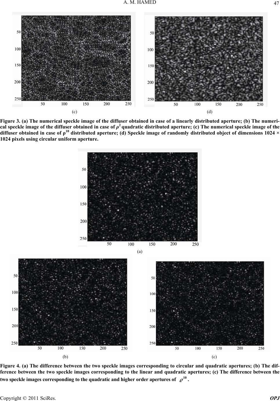

A. M. HAMED
47
(c) (d)
Figure 3. (a) The numerical speed aperture; (b) Thumeri-
cal speckle image of the diffuser obumerical speckle image of the
ckle image of the diffuser obtained in case of a linearly distribut
tained in case of ρ2 quadratic distributed aperture; (c) The n
e n
diffuser obtained in case of ρ10 distributed aperture; (d) Speckle image of randomly distributed object of dimensions 1024 ×
1024 pixels using circular uniform aperture.
(a)
(b) (c)
Figure 4. (a) The difference between the two speckle images corresponding to circular and quadratic apertures; (b) The dif-
ference between the two speckle images corresponding to thear and quadratic apertures; (c) The difference betwe the
two speckle images correspondin
e linen
g to the quadratic and higher order apertures of 10  .

48 A. M. HAMED
(a) (b)
(c) (d)
Figure 5. (a) The profile shape of the numerical speckle mage obtained using the linearly distributed aperture; (b) The profile
shape of the numerical speckle image obtained using the quadratic aperture; (c) The profile shape of the numerical speckle
image obtained in case of ρ10 distributed aperture; (d) The profile shape of the numerical speckle image obtained in case of
uniform circular aperture.
(a) (b)
Figure 6. (a) Reconstruction of the quadratic aperture obtained from the modulated speckle image shown in Figure 3(b); (b)
Reconstruction of the ρ10 aperture obtained from the modulated speckle image shown in Figure 3(c).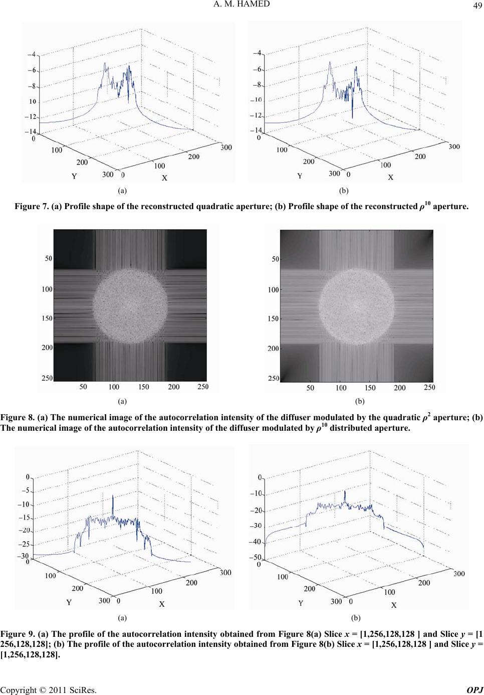

A. M. HAMED
49
(a) (b)
Figure 7. (a) Profile shape of the reconstructed quadratic aperture; (b) Profile shape of the reconstructed ρ10 aperture.
(a) (b)
igure 8. (a) The numerical image of the autocorrelation intensity of the diffuser modulated by the quadratic ρ2 aperture; (b)
The numerical image of the autocorrelation intensity of the diffuser modulated by ρ10 distributed aperture.
F
(a) (b)
Figure 9. (a) The profile of the autocorrelation intensity obtained from Figure 8(a) Slice x = [1,256,128,128 ] and Slice y = [1
256,128,128]; (b) The profile of the autocorrelation intensity obtained from Figure 8(b) Slice x = [1,256,128,128 ] and Slice y =
[1,256,128,128].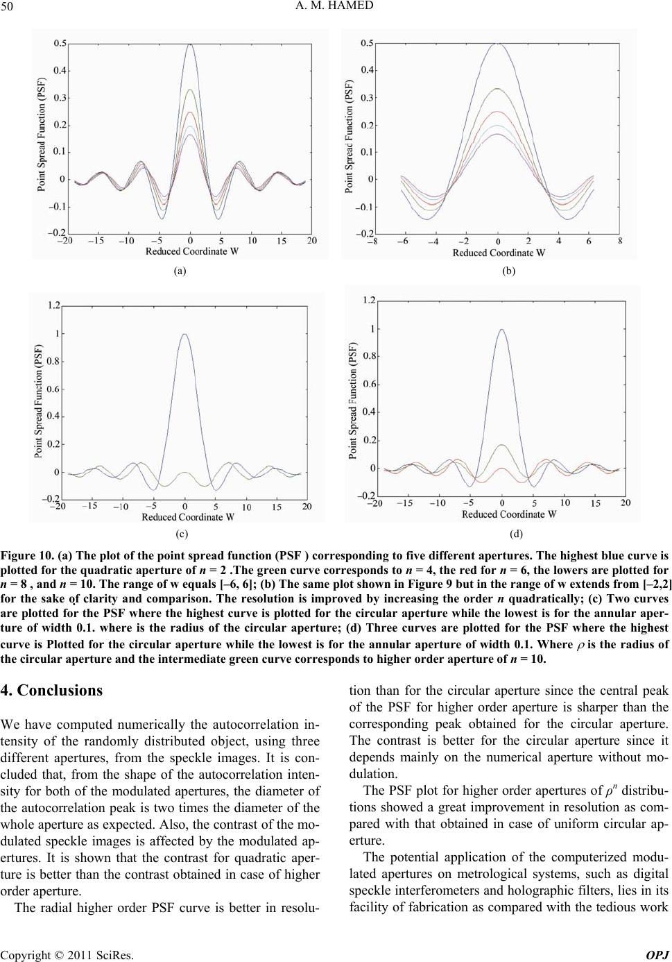

A. M. HAMED
50
(a) (b)
(c) (d)
Figure 10. (a) The plot of the pres. The highest blue curve is
y; (c) Two curves
re plotted for the PSF where the highest curve is plotted for the circular aperture while the lowest is for the annular aper-
ture of width 0.1. where is the radius of the circular aperture; (d) Three curves are plotted for the PSF where the highest
curve is Plotted for the circular aperture while the lowest is for the annular aperture of width 0.1. Where  is the radius of
the circular aperture and the intermediate green curve corresponds to higher order aperture of n = 10.
4. Conclusions
We have computed numerically the autocorrelation in-
tensity of the randomly distributed object, using three
different apertures, from the speckle images. It is con-
cluded that, from the shape of the autocorrelation inten-
sity for both of the modulated apertures, the diameter of
the autocorrelation peak is two times the diameter of the
whole aperture as expected. Also, the contrast of the mo-
dulated speckle images is affected by the modulated ap-
ertures. It is shown that the
her order PSF curve is better in resolu-
tion than for the circular aperture since the central peak
of the PSF for higher order aperture is sharper than the
corresponding peak obtained for the circular aperture.
The contrast is better for the circular aperture since it
depends mainly on the numerical aperture without mo-
dulation.
The PSF plot for higher order apertures of ρn distribu-
tions showed a great improvement in resolution as com-
pared with that obtained in case of uniform circular ap-
erture.
of the computerized modu-
facility of fabrication as compared with the tedious work
oint spread function (PSF ) corresponding to five different apertu
plotted for the quadratic aperture of n = 2 .The green curve corresponds to n = 4, the red for n = 6, the lowers are plotted for
n = 8 , and n = 10. The range of w equals [–6, 6]; (b) The same plot shown in Figure 9 but in the range of w extends from [–2,2]
or the sake of clarity and comparison. The resolution is improved by increasing the order n quadraticallf
a
contrast for quadratic aper-The potential application
ture is better than the contrast obtained in case of higher
order aperture.
The radial hig
lated apertures on metrological systems, such as digital
speckle interferometers and holographic filters, lies in its

A. M. HAMED
51
necessary in thin film techniques.
5. References
[1] J. J. Clair and A. M. Hamed, “Theoretical Studies on
Optical Coherent Microscope,” Optik, Vol. 64, No. 2,
1983, pp. 133-141.
[2] A. M. Hamed and J. J. Clair, “Image and Su-
per-Resolution in Optical Coherent Microscopes,” Optik,
Vol. 64 , No. 4, 1983, pp. 277-284.
[3] A. M. Hamed and J. J. Clair, “Studies on Optical Proper-
ties of Confocal Scanning Optical Microscope Using Pu-
pils with Radial Transmission,” Optik, Vol. 65, No. 3,
1983, pp. 209-218.
[4] A. M. Hamed, “Resolution
Optical Scanning Microscop
nology, Vol. 16, No. 2, 1984, pp. 93-96.
doi:10.1016/0030-3992(84)90061-6
[11] A. M. Hamed, “Numerical Speckle Images Formed by
Diffusers Using Modulated Conical and Linear Aper-
tures,” Journal of Modern Optics, Vol. 56, No. 10, 2009,
pp. 1174-1181. doi:10.1080/09500340902985379
[12] A. M. Hamed, “Formation of Speckle Images Formed For
Diffusers Illuminated by Modulated Aperture (Circular
Obstruction),” Journal of Modern Optics, Vol. 56, No. 15,
2009, pp. 1633-1642. doi:10.1080/09500340903277792
[13] R. D. Bahuguna, “Speckle Patterns of Weak Diffusers:
Effect of Spherical Aberration,” Applied Optics, Vol. 19,
No. 11, 1980, pp. 1874-1878. doi:10.1364/AO.19.001874
[14] H. El-Ghandoor and A. M. Hamed, “Strain Analysis Us-
ing TV Interferometer,” International Symposium on the
Technologies for Optoelectronics Conference, Cannes,
Vol. 683, No. 30, 1987.
lysis of Fringe Contrast
in Electronic Speckle Pattern Interferometer,” Optica
Acta, Vol. 26, No. 3, 1979, pp. 313-327.
[16] G. A. Slettemoen, “Optimal Signal Processing in Elec-
tronic Speckle Pattern Interferometer (ESPI),” Optics
Communications, Vol. 23, No. 2, 1977, pp. 213-216.
doi:10.1016/0030-4018(77)90309-1
and Contrast in Confocal
es,” Optics and Laser Tech-
[5] A. M. Hamed, “A Study on Amplitude Modulation and
an Application on Confocal Imaging,” Optik, Vol. 107
No. 4, 1998, pp. 161-164.
[6] T. Wilson, “Imaging Properties and Applications of
Scanning Optical Microscopes,” Applied Physics, Vol. 22,
No. 2, 1980, pp. 119-128. doi:10.1007/BF00885994
[7] C. J. R. Sheppard and A. Choudhary, “Image Formation
in the Scanning Microscope,” Journal of Modern Optics,
Vol. 24, No. 10, 1977, pp. 1051-1073.
[8] G. Nomarski, The Journal of the Optical Society of
America. Vol. 65, No. 10, 1975, p. 1166.
[9] C. J. R. Sheppard and T. Wilson, “Image Formation In
Scanning Microscopes with Partially Coherent Source
and Detector,” Journal of M odern Optics, Vol. 25, No. 4,
1978, pp. 315-325.
[10] I. J. Cox, C. J. R. Sheppard and T. Wilson, “Improvement
in Resolution by Nearly Confocal Microscopy,” Applied
Optics, Vol. 21, No. 5, 1982, pp. 778-781.
doi:10.1364/AO.21.000778
[15] G. A. Slettemoen, “General Ana
[17] R. S. Sirohi and A. R. Ganesan, “Holographic Systems,
Components and Applications,” Proceedings of the 2nd
International Conference on IEEE, 1989.
[18] Y. Z. Song and H. L. Zhang, etc., “Dynamic Digital
Speckle Interferometry Applied to Optical Diagnosis of
Gas-Liquid Phase Change,” The International Society for
Optical Engineering, Vol. 4448, 2009, pp. 111-119.
[19] C. Greated, E. Lavinskaya and N. Fomin, “Numerical
Simulation of Acoustical Wave Tracing,” Journal of
Mathematical Modelling, Russian Academy of Science,
. Vol. 15, No. 7, 2003, pp. 75-80
[20] J. W. Goodmann, “Introduction to Fourier Optics and
Holography,” McGraw-Hill book Company, New York,
1968.
[21] J. D. Gaskill, “Linear Systems, Fourier Transforms, and
Optics,” John Wiley &Sons, Inc., New York, 1978.