Journal of Quantum Information Science, 2011, 1, 18-25
doi:10.4236/jqis.2011.11003 Published Online June 2011 (http://www.SciRP.org/journal/jqis)
A Numerical Study of the Flow with Heat Transfer of a
Pseudoplastic Fluid between Parallel Plates
S. Iqbal1, A. Zeb2, A. M. Siddiqui3, Tahira Haroon4
1Department of Com p ut er Sci ence, COMSATS Institute of Information Technology, Sahiwal Campus,
Sahiwal, Pakistan
2Department of Mat hem at i cs, Faculty of Science, Al-Imam Ibn Saud University,
Riyadh, Saudi Arabia.
3Department of Mat hem at i cs, Pennsylvania State University, York Campus, York , USA
4Department of Mat hem at i cs, COMSATS Institute of Information Technology,
Islamabad, Pakistan
Received April 26, 2011; revised May 25, 2011; accept e d June 5, 2011
Abstract
One dimensional flow with heat transfer of a pseudoplastic fluid between two infinite horizontal parallel
plates is investigated. The thermophysical properties of the fluid are assumed to be constant and numerical
solution using the finite element method, along with the corresponding exact solution for the fluid velocity
and the fluid temperature is obtained. The effect of variation of the governing parameters is studied using
figures and tables. It is found that the numerical solution agrees well with the corresponding exact solution
and that the fluid velocity, together with the fluid temperature, increases with increasing values of the
governing parameters.
Keywords: Pseudoplastic Fluids, Heat Transfer, Finite Element Method, Exact Solution
1. Introduction
Over the past few decades there has been a growing
recognition of the fact that many fluids of industrial
significance do not obey the Newtonian postulate of
linear relationship between the shear stress and shear
rate. Therefore, these fluids are known as non-
Newtonian fluids. Common examples of such fluids are
slurries, pastes, gels, molten plastics and lubricants
containing polymer additives. Various food stuffs such
as honey and tomato sauce, the biological fluids like
blood and synovial fluid naturally found in cavities of
synovial joints also belong to the general class of the
non-Newtonian fluids [1,2]. The simplest model of
non-Newtonian fluids is the power law model and a
special case of the power law equation, with , is
the pseudoplastic model. Commonly encountered non-
Newtonian fluids like polymer solutions, paper pulps,
detergents, oils and greases may be classified by the
pseudoplastic fluid model [3]. The pseudoplastic fluids
represent shear thinning fluids, and as far as we know,
this class of non-Newtonian fluids received less
attention in the literature.
<1n
Heat transfer processing of non-Newtonian fluids is
one of the key components of the flow phenomenon in
various industrial sectors including chemicals, petro
chemicals, food industry, polymers and pharmaceuticals
[3-6]. Therefore, in the present paper we consider
one-dimensional steady laminar flow, with heat transfer,
of a pseudo plastic fluid between two fixed infinite
horizontal parallel plates. The fluid motion is generated
by the presence of a constant external pressure gradient
along x-axis and the fluid velocity components along y-
and z-directions are zero. Thus, the momentum equations
break down to a second order ordinary differential equation
and we need two boundary conditions for finding a
solution to this equation. These boundary conditions are
obtained from the no slip condition and the condition of
symmetry at the center line of the flow channel. We
integrate the resulting momentum equation once in
combination with the condition of symmetry to obtain a
quadratic equation in th e unknown shear rate dduy.
We apply the Finite Element Method (FEM) to solve
this quadratic equation numerically and compare the
numerical solution with the co rresponding exact solution
of the equation. For details on the implementation of the

S. IQBAL ET AL.
19
FEM the interested reader may consult from the
references [7-10]. To find exact solution of the problem,
we follow the approach used by Deiber and Santa Cruz
[11] and find two values of the shear rate by
solving the resulting quadratic equation. However, we
retain only one of these two values as the other does not
satisfy the condition of symmetry. Then a second
integration of
/du dy
dduy in combination with the no-slip
condition provides an exact so lu tion for the fluid velocity.
Once the fluid velocity solu tion is known, we may use it
to find solution for the fluid temperature from the
resulting energy equ a tion.
The following discussion begins with the basic equations,
governing the flow of an incompressible fluid, in section 2.
The problem is, respectively, formulated and solved in
sections 3 and 4. Results obtained from the numerical and
exact solutions for various values of the governing
parameters are presented and discussed in section 5. Finally
some conclusions are mentioned in section 6.
2. Basic Equations
The basic e qua ti ons gove r ni ng the flo w of an in com pre ssi ble
fluid are given by the laws of the conservation of mass,
the conservation of momentum and the conservation of
energy, see [1,2]
= 0u (1)
=
D
Dt
 
ufT (2)
2
=
pD
CDt 
 TL
(3)
where u is the velocity field, f is the body force, T is the
stress tensor, is the fluid tem perat ure, 

is the constant
fluid density, is the thermal conductivity,

p
C is the
specific heat, L is the gradient of u and DDt is the
material derivative. The stress tensor T for pseudo plastic
fluid is defined by the constitutiv e equations, see [2].
=pTIS (4)
where p is the reaction stress due to the constraint of
incompressibility. The extra stress tensor S is defined by
the expression, see [11]
 
11111
1=
2o
 

 1
S
SASSAA (5)
where o

is the zero shear viscosity, 1

is the
relaxation time and 1

is the material constant. The first
Rivlin-Ericksen tensor 1 is defined as 1
A=T

A
LL
and the contravariant convected derivative denoted by
superimposed over S is defined as 
=T
t




 



 

S
uSLSSL (6)
3. Problem Formulation
We consider one-dimensional heat transfer flow of pseudo
plastic fluid between two infinite horizontal parallel
plates distant apart. The flow is produced by a
constant external pressure gradient
2hddpx, the
temperature of the upper plate is maintained at 1

and
that of the lower plate at o. The fluid moves in the 
x
direction

parallel to the plates and there is no
velocity in
y
and z dsirection

. Thus, equation (1)
implies =0
u
x

, which means . Hence, the

=uuy
fluid velocity field and the temperature distribution are
assumed to be of the following form


 
=,0,0,= ,=uuuyuy (7)
Then, the continuity Equation (1 ) is satisfied identically,
the material derivative Du
Dt vanishes and, in the absence
of body forces, the momentum Equation (2) reduces to
=0

T. This leads to the following second order
equation


2
0
2
d/d
dd
()= ,=
dd1d/d
xy xy
uy
p
SS
yx uy

  (8)
where


22
11
=



. The boundary conditions,
respectively, obtained from the no slip condition and the
condition of symmetry are and

=0uh


0=0
xy
S.
Integrating Equation (8) once and applying


0=0
xy
S
yields
2
dd
=0
dd
o
uu
Py Py
yy




 (9)
where P

denotes the constant pressure gradient
ddpx. Similarly, using (7), we see that /=0DDt,

22
=d 2 /d
y

=
xy
S y

P
and xy . Moreover,
the Equation (8) and the condition xy generate

=d/SuTL

S

dy
0=0

. Therefore, the energy Equation (3) reduces
to the equation
2
2
dd
=0
d d
u
Py y
y

 (10)
and the boundary conditions on  are (–h) = 

0
and


h=

1, which are provided by the fluid
temperature on the plates. For non-dimensionalization of
Equations (9) and (10), we introduce the following
dimensionless variables.

20 S. IQBAL ET AL.
2
2*
1
1
=, =,=,=,=
uyPhU
uyP
Uh Uh


 
 



(11)
where 0 is the bulk mean temperature and U is a
typical fluid velocity. After omitting asterisks, the
Equations (9) and (10) can be written in their respective
dimensionless form as follows

2
dd =0
dd
uu
Py Py
yy




 (12)
2
2
dd
=0
d d
u
yP
y y

 (13)
where
 
22
11
== =
p
p
c
UUPrEc
c




 



is
the Brinkman number, is the Prandtle and is
the Eckert number. Finally, non-dimensionalising the
remaining boundary condition on u and the two boundary
conditions on  we obtain , and
.
Pr Ec
0

1=0u

1=

1=1
4. Solution of the Problem
In this section we apply the FEM to solve Equation (12)
subject to and the resulting energy Equation
(13) subject to the boundary conditions and
for finding fluid velocity and temperature
fields, respectively. We also find exact solution for the
sake of comparison.

1=0u
0

1=0

1=
4.1. Fluid Velocity
Clearly, for the choice =0

, the Equation (12) reduces
to the corresponding equation for viscous flow. Therefore,
in order to maintain non-newto nian character istics of the
velocity Equation (12), we assume that 0

.
The Galerkin’s finite element method provides an
elegant approach for constructing approximations of
solutions of boundary value problems. It provides a
general and precise procedure for constructing basis
functions. The main idea is that the basis functions can
be defined piecewise over sub-regions of the domain
called finite elements and that over any sub-domain, the
basis functions can be chosen to be very simple functions
such a polynomials of low degree. Therefore, the
Galerkin’s formulation in the finite element fashion
requires, see [7-10], that we choose a suitable trial or
basis approximation V to the true solution V that is
applied locally over a typical finite element in the
complete y domain. The simplest such solution is linear
trial function, . From finite element
analysis, rather than formulating the problem in terms of
arbitrary constants 1 & 2, we prefer to recast the
bove linear trial function in terms of values of the
dependent functions at nodes i & j [7,8],

1
Vaa2 =y

a
12
a

 
=T
ij
VNVNV NV
 (14)
Here


=,
i
VV
j
V



 is a vector of the nodal variables
and




1
=,NNN
2
is a vector of the interpolation or
shape functions with
 
1
j
ji
and
=Nyyyy




2i
are called linear Lagrange
interpolation polynomials, now are the nodal values of
the dependent variable .
=ij Nyyyy
''
nn

V

Now applying quasi-liberalization, see [12], to first of
the governing system of differential Equation (12) and
(13), we obtain
11 n
u  2
''
n
uPyuuPy 

  2=0 (15)
We follow the standard Galerkin’s approach and
choose the weighting function .
Now integrating over the entire region, we get

=,=1,2
''
i
wy Ni



2
'' ''
nnnn
YwyuPyuuPyy

11
2
'
u

d=0 
(16)
where 'd/dy

. For our particular problem, after
substituting the trial functions in Equation (16), we have
the following discretised form


=1
d2dd2 d
=0
n'''''' '
nnnn
YY
e
wuywuywuyPwy y  


11
'
u y


YY
P


(17)
where e stands for element and n represents the total
number of elements in the discretised region. In matrix
notation, the system of Equations (17) can be written as

=1
1=f0,
1
1
=,=
1
n
e
kf
L



11
11
ku 











(18)
where k is a stiffness matrix and f is a force vector, =



i
yand =
nn
ij j
uu   Py . Applying the assembly
procedure given in the references [7-10] and using
Equation (18) for n elements, we get

1
2
3
1
110
1
2
0
1
12
0 1
12 0 00
01 0
1=
00 0
1 0
000 111
n
n
u
u
u
L
u
u
 


 





 







 




 













 














(19)

S. IQBAL ET AL.
21
The solution of the system (19) provides the numerical
solution of Equation (12) for fluid velocity profile. The
final arrangement of the stiffness matrix (19) is
noteworthy, nonzero entries come into sight clustered
near the main diagonal of the matrix. Outside this band
of nonzero terms, all entries are zero. Matrices of this
type are said to be banded. Also, it is seen in (19) that the
stiffness matrix is symmetric, though we shall not always
have symmetry, nevertheless in most physical problems
based on conservation laws this symmetry will arise
quite naturally. This symmetry will always be possible to
attain in self-adjoint boundary value problem. These two
properties of stiffness matrices play a vital role in the
stratagem of programming finite element calculations.
For finding the exact solution of the Equation (12) we
solve this equation for dduy and obtain
22
114
d=
d2
Py
u
yPy


  (20)
We retain only one of the roots (20) because the other does
not satisfy the condition of symmetry and write

0=0
xy
S
22
14 1
d=
d2
Py
u
yPy



(21)
Integrating Equation (21) in combination with the
boundary condition yields the fluid velocity
solution

1=0u
2
22 2
22
=
14 1 11414 ln
214 1
u
P
Py P
PPy




















(22)
Equation (22) is exact solution for the fluid velocity.
Clearly this expression for the fluid velocity can have a
physical meaning if it is defined only in the set of real
numbers. Therefore, the solution given by Equation (22)
is physically valid provided the condition 2 41P 

is
satisfied. This further means that, if the pressure gradient
P is fixed, the parameter

should be strictly set in the
range . Similarly, if the parameter
2
0< <1/4P 

is
fixed at a positive value the P should take a value that
ensures validity of th e condition 0< <12P

.
4.2. Fluid Temperature
Now, using the fluid velocity solution obtained from the
system (19) and applying the same Galerkin’s FEM
formulation to the second of the system of governing
differential Equations (12) and (13), we get

=1
dd
n'' '
n
YY
e
wyPwyuy  


which in matrix notation, can be written as

11
=1
2
=0,=2
6
n
j
i
e
j
i
yy
PL
kf fyy



 



(24)
where 1
f
is a force vector. By applying the assembly
procedure given in [7-10], and using (23) for n elements,
we get



1
2
3
1
1100 0
12 100
0121
1
00 0
12 1
000 11
2
3
3
=6
3
2
n
n
ji
ji
ji
ji
ji
L
yy
yy
yy
PL
yy
yy


 



 




 











 
























 





(25)
The solution of the system (25) gives us the temperature
distributions of the flow by imposing the boundary
conditions.
Next, for evaluation of the temperature distribution,
we substitute the fluid velocity solution (22) in the
Equation (13) to obtain


222
2
d14 1=0
2 dPy y


 
(26)
provided the condition is satisfied. Now
integrating Equation (26) twice and applying the boundary
conditions
2
4P  1


1=0 and , we arrive at the
following exact solution for the fluid temperature.

1= 1

123
1
=( )1
22
y




  (27)
Where
 


3/2 3/2
22
12
1
1
=1414
24 PPy P



2
(28)

11
21
=(2)(2
sin sin
4yPy P



)P  (29)


2
22 2
32
1
11
=14 142
8
y
Py P
P



 (30)
=0, (23) provided 2
41P 

.

S. IQBAL ET AL.
22
5. Results and Discussion parameters

and P is presented in Figure 1(b). A
satisfactory agreement of numerical solution with the
corresponding exact solution may be observed from
these figures. In Table 1 we show variation of the
As mentioned earlier, for a fixed P, the parameter

is
strictly set in the range 2
0< 14P  . Again, for a
fixed

, P must obey the restriction 0< 12absolute error =
uFEMExact
Eu u for and =0.5P
P

.
Therefore, if we choose =1 2P, then the value of the
parameter

should lie in the range 0< 1


.
Similarly if the non-Newtonian parameter is taken to be
=14
values of


0.4, 0.6, 0.8  E. From this table we observe
that size of the error u is sufficiently small to confirm
agrement of the numerical solution with the corresponding
exact solution. Furthermore, we observe from Figures
1(a) and 1(b) that the fluid velocity magnitude increases
with increasing values of the non-Newtonian parameter

.

then the value of P must fall in the range
. 0<P1
In Figure 1(a) we present the fluid velocity solution
obtained by solving Equation (12) by applying the finite
Figure 2(a) presents the FEM solution with the fluid
velocity for =0.25

and various values of P



0.4,0.6,0.8 and Figure 2(b) shows the exact solution
element method for and various values of
. The corresponding exact solution (22)
=0.5P

0.4,0.6,0.8  
for the fluid velocity with same values of the
(a) (b)
Figure 1. Effect of varying β on (a) the FEM solution; (b) the exact solution for the fluid velocity, when P = 0.5.
(a) (b)
Figure 2. Effect of varying P on (a) the FEM solution; (b) the exact solution for the fluid velocity, when β = 0.25.

S. IQBAL ET AL.
23
(a) (b)
Figure 3. Effect of varying P on (a) the FEM solution; (b) the exact solution for the fluid temperature, when β = 0.25 and

= 5.
(a) (b)
Figure 4. Effect of varying

on (a) the FEM solution; (b) the exact solution for the fluid temperature, when β = 0.25
and P = 0.8.
Table 1. Variation of Eu for P = 0.5 and various values of β.
y
0.4=

0.6=

0.8=

0.2 6
103.6823   6 107.6414   5 101.7170  
0.4 6
103.3612   6 107.1423  5 101.6480  
0.6 6
102.7609   6 106.1459   5 101.4999  
0.8 6
101.7458  6 104.2353  5 101.1671  
Table 2. Variation of Eu with β = 0.25 and various values of P.
y 0.4=P 0.6=P 0.8=P
0.2 7
108.8982   6 103.7714   5 101.4155 
0.4 7
107.9124   6 103.4271   5 101.3297  
0.6 7
106.1969   6 102.7912   5 101.1560  
0.8 7
103.6284   6 101.7396   6 108.1334  
Table 3. Variation of Θ
E
with β = 0.25, =5

and vari-
ous values of P.
y
0.1=P 0.6=P 0.9=P
0.2 9
101.0486   6 101.7861   5 101.6398 
0.4 9
101.0236   6 101.7525  5 101.6218 
0.6 10
109.1504   6 101.5969   5 101.5307  
0.8 10
106.2155   6 101.1338  5 101.2060  
Table 4. Variation of Θ
E
with β = 0.25, P = 0.5 and
various values of

.
y
1.0


3.0

 5.0


0.2 6
101.5414   6 104.6242   6 107.7071  
0.4 6
101.5194   6 104.5583  6 107.5971  
0.6 6
101.4121   6 104.2362   6 107.0603 
0.8 6
101.0581   6 103.1743  6 105.2904  

24 S. IQBAL ET AL.
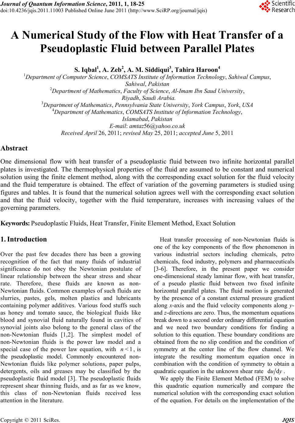
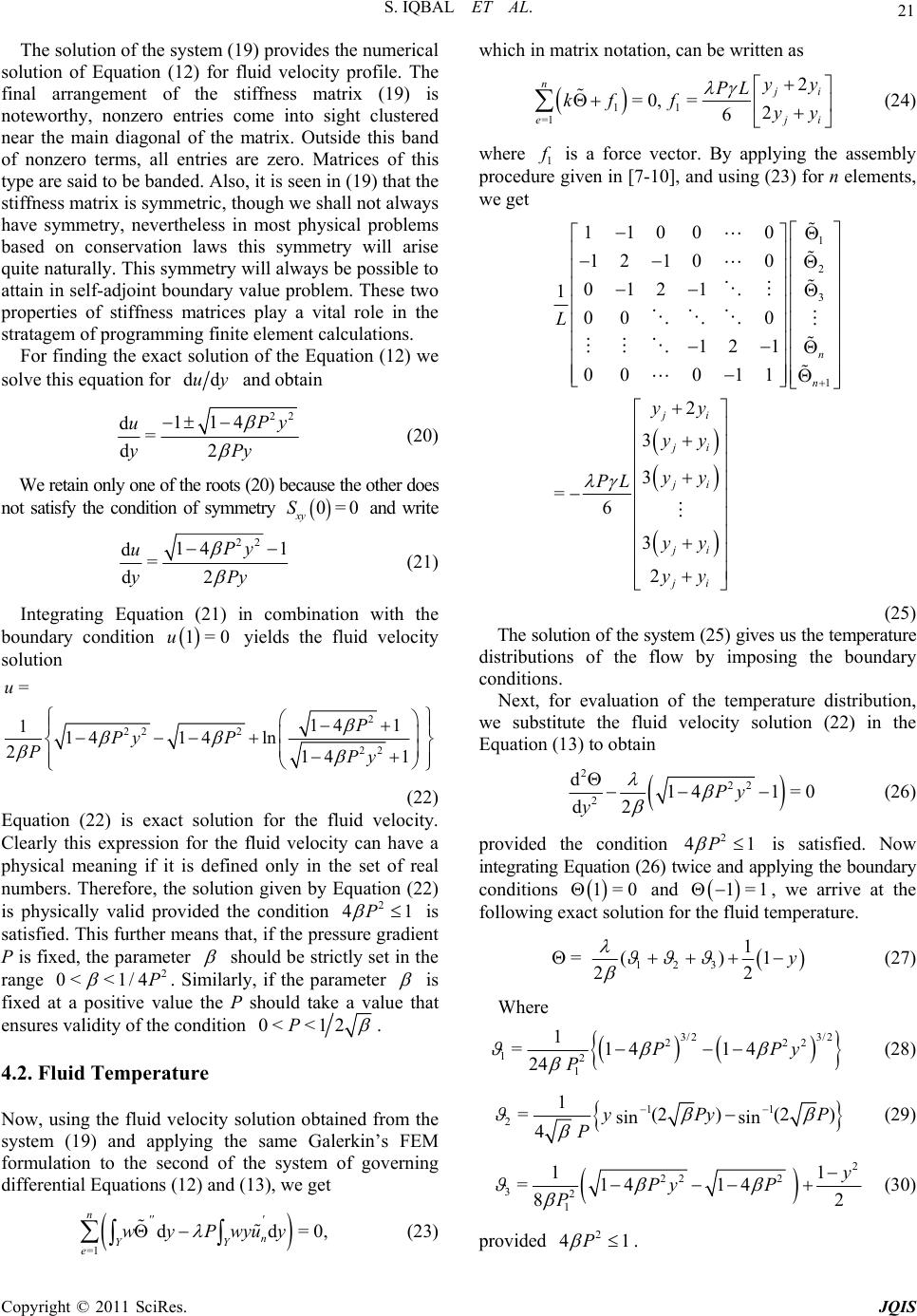
(22) for the fluid velocity with same values of

and P.
From these figures we observe that the agreement of the
numerical solution with the co rresponding exact solution
is very good. This agreement is further highlighted by
sufficiently small size of the absolute error shown
in Table 2 for u
E
=0.25

and . The
fluid velocity magnitude again appears to show an
increasing trend with increasing values of the pressure
gradient P. Thus we conclude that the fluid velocity
magnitude increases with increasing values of the non-
Newtonian parameter

0.80.4, 0.6,P

and the pressure gradient P,
when one of these is fixed.
Figure 3(a) illustrates variation of the numerical
solution for the fluid temperature obtained by the finite
element method with = 0.25,= 5



0.9 and various values of . The corresponding exact
solution is presented in Figure 3(b) for same values of
the parameters

0.1,0.6 ,P

and P. From these figures we observe
that the numerical sol uti on for the fluid tem pe r ature e x hibits
good agreement with the corresponding exact solution.
This agreement of the numerical solution with exact
solution is further illustrated in Table 3. This table presents
variation of the absolute error =
F
EM Exact
E for
=0.25, =5

 P and . It may be
observed from this table that the size of the error

0.1,0.6 ,0.9

E

is
small enough to illustrate accuracy of the numerical
solution. Moreover, we observe that the fluid temperature
increases with increasing values of P for fixed

and

are fixed.
Then in Figure 4(a) we present variation of the FEM
numerical solution for =0.25, =0.5P

and

1.0,3.0,5.0  
6. Conclusions
One dimensional flow of a constant property pseudo
plastic fluid with heat transfer between two infinite
horizontal parallel plates is considered. Numerical
solutions for the dimensionless fluid velocity and the
fluid temperature are obtained by applying the finite
element method. The corresponding exact solutions are
also derived for the sake of comparison. It is found that
the numerical technique based on the finite element
method produces highly accurate solution both for the
fluid velocity and the fluid temperature that agrees nicely
with the corresponding exact solution. Moreover, the
fluid velocity along with the fluid temperature increases
with increasing values of the pressure gradient P, the
non-Newtonian parameter

and/or the Brinkman
number

.
7. References
[1] G. Astarita and G. Marrucci, “Principles of Non-
Newtonian Fluid Mechanics,” McGraw Hill, London,
1974.
[2] R. B. Bird, R. C. Armstrong and O. Hassager, “Dynamics
of Polymeric Liquids, Fluid Mechanics,” Wiley, New
York, 1987.
[3] M. Moradi, “Laminar Flow Heat Transfer of a
Pseudoplastic Fluid through a Double Pipe Heat
Exchanger,” Iranian Journal of Chemical Engineering,
Vol. 3, No. 2, 2006, pp. 13-19.
[4] M. Massoudi and I. Christie, “Effects of Variable
Viscosity and Viscous Dissipa tion on the Flow of a Third
Grade Fluid in a Pipe,” International Journal of
Non-Linear Mechanics, Vol. 30, No. 5, 1995, pp.
687-699.
doi:10.1016/0020-7462(95)00031-I

. The corresponding exact solution for
the same values of the parameters ,

 and P is
presented in Figure 4(b) for the sake of comparison.
From these figures we again observe that the agreement
of the numerical solution for the fluid temperature with
the corresponding exact solution is very good. We
present the absolute error E

for = 0.25,

and in Table 4 and observe that the
size of is satisfactorily small to confirm agreement
of the numerical solution with the corresponding exact
solution. Moreover, as we see from Figure 4, again the
fluid temperature shows an increasing trend with
increasing values of
=0.5P

1.0,3.0,  E
[5] A. M. Siddiqui, A. Zeb, Q. K. Ghori and A. M.
Benharbit, “Homotopy Perturbation Method for Heat
Transfer Flow of a Third Grade Fluid between Parallel
Plates,” Chaos Solitons and Fractals, Vol. 36, No. 1,
2008, pp. 182-192.

5.0

, when P and

are held fixed.
Further, we report without presenting that the numerical
solution for the fluid temperature and the
corresponding absolute error shows similar
behavior with varying

E

and fixed P and

. Therefore,
we conclude that the fluid temperature increases with
increasing values of the non-Newtonian parameter

,
the Brinkman number

and the pressure gradient P,
when any two of these parameters are held fixed.
[6] T. Hayat, K. Maqbool and M. Khan, “Hall and Heat
Transfer Effects on the Steady Flow of a Generalized
Burger's Fluid Induced by Sudden Pull of Eccentric
Rotating Disks,” Nonlinear Dynamics, Vol. 51, No. 1-2,
2008, pp. 267-276. doi:10.1007/s11071-007-9209-2
[7] F. L. Stasa, “Applied Finite Element Analysis for
Engineers, ” CBS Publishing, 1985.
[8] O. C. Zienkiewicz, “The Finite Element Method,”
McGraw Hill, London, 1977.
[9] S. Iqbal, A. M. Mirza and I. A. Tirmizi, “Galerkin’s
Finite Element Formulation of the Second-Order
Boundary-Value Problems,” International Journal of
Computer Mathematics, Vol. 87, No. 9, 2010, pp.
2032-2042.

S. IQBAL ET AL.
25
doi:10.1080/00207160802562580
[10] S. Iqbal and N. A. Memon, “Numerical Solution of
Singular Two-Point Boundary Value Problems Using
Galerkin's Finite Element Method,” Quaid-e-Awam
University Research Journal of Engineering, Science
and Technology (QUEST-RJ), Vol. 9, No. 1, 2010, pp.
14-19.
[11] J. A. Deiber and A. S. M. Santa Cruz, “On Non-Newtonian
Fluid Flow through a Tube of Circular Cross Section,”
Latin American Journal of Chemistry Engineering and
Applied Chemistry, Vol. 14, 1984, pp. 19-38.
[12] R. E. Bellman and R. E. Kalaba, “Quasilinearizalion and
Nonlinear Boundary-Value Problems,” American E lse vie r,
New York, 1965.