Journal of Quantum Informatio n Science, 2011, 1, 7-17
doi:10.4236/jqis.2011.11002 Published Online June 2011 (http://www.SciRP.org/journal/jqis)
Application of Scale Relativity (ScR) Theory to the
Problem of a Particle in a Finite One-Dimensional Square
Well (FODSW) Potential
Saeed Naif Turki Al-Rashid1*, Mohammed Abdul-Zahra Habeeb2, Khalid Abdulwahab Ahmed3
1Physics Department, College of Science, Al-Anbar University, Anbar, Iraq
2Physics Department, College of Science, Al-Nahrain University, Baghdad, Iraq
3Physics Department, College of Science, Al-Mustansiriyah University, Baghdad, Iraq
Received April 16, 2011; revised May 22, 2011; accepted June 1, 2011
Abstract
In the present work, and along the lines of Hermann, ScR theory is applied to a finite one-dimensional square
well potential problem. The aim is to show that scale relativity theory can reproduce quantum mechanical
results without employing the Schrödinger equation. Some mathematical difficulties that arise when obtain-
ing the solution to this problem were overcome by utilizing a novel mathematical connection between ScR
theory and the well-known Riccati equation. Computer programs were written using the standard MATLAB
7 code to numerically simulate the behavior of the quantum particle in the above potential utilizing the solu-
tions of the fractal equations of motion obtained from ScR theory. Several attempts were made to fix some of
the parameters in the numerical simulations to obtain the best possible results in a practical computer CPU
time within limited local computer facilities. Comparison of the present results with the corresponding re-
sults obtained from conventional quantum mechanics by solving the Schrödinger equation, shows very good
agreement. This agreement was improved further by optimizing the parameters used in the numerical simu-
lations. This represents a new example where scale relativity theory, based on a fractal space-time concept,
can accurately reproduce quantum mechanical results without invoking the Schrödinger equation.
Keywords: Square Well, ScR Theory, Numerical Simulations, Fractal Space-Time
1. Introduction
The extension of the principle of relativity gives new
theory of relativity, which is the scale relativity (ScR)
theory as introduced by Nottale [1-3] in 1993. This the-
ory states that: “the fundamental laws of nature apply
whatever the state of scale of the coordinate system”.
The state of a reference system is characterized by the
resolutions at which this system is observed. It can be
defined only in a relative way. The main idea of ScR
theory is to give up the arbitrary hypothesis of differen-
tiability of space-time. This theory reformulated quantum
mechanics from first principles leading to the covariance
and geodesic equations by considering a particle as a
geodesic in fractal space-time. ScR theory applies in the
three domains of microphysics, cosmology and complex
systems [2-9].
As far as quantum mechanics is concerned, Nottale
and co-workers were able to apply the theory to solve
many problems, especially those related to the concep-
tual and interpretation aspects. In this connection, we
mention the work on the derivation of the postulates of
quantum mechanics from the first principles of the ScR
theory [10]. In terms of the results of this work, all
quantum mechanics and not only the Schrödinger equa-
tion, arises as a direct consequence of the fractality of
space-time. The extension of the ScR theory to the deri-
vation of the main equations of relativistic quantum me-
chanics [11] and the relationship between the classical
and quantum regimes [12] have been also discussed on
the basis of the ScR theory, among other important con-
sequences and implications. With all these far reaching
aspects of the theory, direct investigations which would
shed light on the basic workings of the ScR theory as
formulated by Nottale seem to be warranted.
In this regard, Hermann [13] was the first, and to our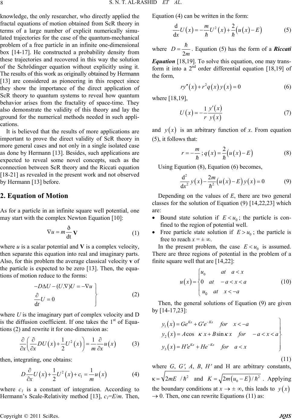

8 S. N. T. AL-RASHID ET AL.
knowledge, the only researcher, who directly applied the
fractal equations of motion obtained from ScR theory in
terms of a large number of explicit numerically simu-
lated trajectories for the case of the quantum-mechanical
problem of a free particle in an infinite one-dimensional
box [14-17]. He constructed a probability density from
these trajectories and recovered in this way the solution
of the Schrödinger equation without explicitly using it.
The results of this work as originally obtained by Hermann
[13] are considered as pioneering in this respect since
they show the importance of the direct application of
ScR theory to quantum systems to reveal how quantum
behavior arises from the fractality of space-time. They
also demonstrate the validity of this theory and lay the
ground for the numerical methods needed in such appli-
cations.
It is believed that the results of more applications are
important to prove the direct validity of ScR theory in
more general cases and not only in a single isolated case
as done by Hermann [13]. Besides, such applications are
expected to reveal some novel concepts, such as the
connection between ScR theory and the Riccati equation
[18-21] as revealed in the present work and not observed
by Hermann [13] before.
2. Equation of Motion
As for a particle in an infinite square well potential, one
may start with the complex Newton Equation [10]:
ð
dt
um V (1)
where u is a scalar potential and V is a complex velocity,
then separate this equation into real and imaginary parts.
Also, for this problem the average classical velocity v of
the particle is expected to be zero [13]. Then, the equa-
tions of motion reduce to the forms:
(.)
0
d
DUUU u
U
t
 




(2)
where U is the imaginary part of complex velocity and D
is the diffusion coefficient. If one takes the 1st of Equa-
tions (2) and rewrite it for one-dimension as:
 
2
11
2
DUxUxu x
xx mx
 



 

(3)
then, integrating, one obtains:
  
2
1
11
2
DUx Uxcux
xm

 (4)
where c1 is a constant of integration. According to
Hermann’s Scale-Relativity method [13], c1=E/m. Then,
Equation (4) can be written in the form:
  
2
d2
d
m
UxU xuxE
x



 (5)
where 2 Dm . Equation (5) has the form of a Riccati
Equation [18,19]. To solve this equation, one may trans-
form it into a 2nd order differential equation [18,19] of
the form,




20ryxr qxyx


 (6)
where [18,19],




1yx
Ux ryx

 (7)
and


y
x is an arbitrary function of x. From equation
(5), it follows that:
m
r

;
  
2
qxux E



 (8)
Using Equation (8), Equation (6) becomes,
 


2
22
d2 0
d
m
yxux Eyx
x



x
(9)
Depending on the values of E, there are two general
classes for the solution of Equation (9) [14,22,23] which
are:
 Bound state solution if 0 Eu; the particle is con-
fined to the region of potential well.
 Free particle state solution if 0 Eu; the particle is
free to reach x = ± .
In the present problem, the case 0 is assumed.
There are three regions of potential in the problem of a
finite square well that are [14,22]:
Eu

0
0
uata
uxatax a
uatx a
 





0
(10)
Then, the general solutions of Equation (9) are given
by [14-17,23]:



1
2
3
cos sin
Kx Kx
Kx Kx
yxGeGefor xa
yxAxBx foraxa
yxHeHefora x




  


 





 
(11)
where G, G
 , A, B, H  and H are arbitrary constants,
κ2 2/mE and

2
0
2KmuE/. Applying
the boundary conditions at x  ± , this leads to


y
x
 0. Then, one can rewrite Equations (11) as:

S. N. T. AL-RASHID ET AL.
9



1
2
3
cos sin
Kx
Kx
yx Ge
yx AxBx
yx He










(12)
The next step is to apply the matching conditions at
the boundaries between regions, which require that both
function and its derivative be continuous. In this way,
one gets a set of four homogeneous linear equations with
four unknowns [19]:
(1)
cos sin
sin cos
Kx
Ka
GeAa Ba
f
or xa
KGeAa Ba

 



 





(13)
(2)
cos sin
sin cos
Ka
Ka
AaBaHe
f
or xa
AaB aKHe

 



 



 

(14)
These equations can be rewritten in matrix form as:
cos sin0
sin cos00
cossin 0
coscos 0
Ka
Ka
Ka
Ka
aae AA
aaKeBB
GG
aa e
HH
aaKe

 









 

 


 


 

 

 



M
(15)
where the matrix M is given by:
cos sin0
sin cos0
cossin 0
cos cos0
Ka
Ka
K
a
K
a
aae
aaKe
aa e
aaKe

 


















M









(16)
The trivial solution of Equation (15) is A = 0, B = 0, G
= 0 and H = 0 [23]. While, for a non-trivial solution to
exist, the condition [23]:
detM = 0 (17)
must be satisfied. To simplify, one eliminates the coeffi-
cients G and H. Then, Equation (15) becomes the 2 × 2
matrix equation [23]:
0
tantan
tantan 






























B
A
M
B
A
aKKa
aKKa


(18)
For this equation to have a non-trivial solution, the de-
terminant of the coefficients must be equal to zero, or:




2tantan 0aK Ka  

 (19)
Then, there are two solutions which are [23]:
(a) κ tan κ=K, this means B =0 and
a


2cos
y
xA x   (20)
(b) K tan κ= κ, this means A = 0 and
a


2sin
y
xB  x (21)
Equation (20) corresponds to even parity solutions
while Equation (21) corresponds to odd parity solutions.
These equations can be simplified by introducing the
new dimensionless variables:
x
a


and

= K (22)
a
From the definition of κ and K, one can write:
22
0
2
2m
K
u  
 (23)
Using Equation (22), one can rewrite Equations (20),
(21) and (23) in the forms:

=
x
tan
x
(24)

= –
x
cot
x
(25)
22 2
2
2m
xua
2





 (26)
where the dimensionless parameter  measures the vol-
ume of the potential in unit of ħ2/2 m.
2
0
ua
To determine the values of κ and K in Equations (24)
and (25), one may solve these equations graphically
together with Equation (26) [14-17,22,23].
Figures (1) and (2) give the intercepts for the even
parity solution (Equation (24)) and the odd parity
solution (Equation (25)) for two sets of values of the
potential volume parameter ( = 1 and 4) and ( = 2 and
6) for the even and odd parity solutions respectively. In
these figures, κ is drawn horizontally and

vertically.
The dashed curve is that of
x
tan
x
(for even parity) or
x
cot
x
(for odd parity). The continuous curve is that of
22
x2




The values of κ and K (x and

) corresponding to the
solutions of Equations (24), (25) and (26) can be deter-
mined from Figures (1) and (2). Then, one can calculate
the state energy and the function for different val-
ues of  in the following way:
)(xy
(1) For
 =1 (equivalent to n = 1), x  0.7391 and

=
0.673. This is called the ground state energy, which is:

22
2
2
0.7391 0.273
2
gs
Ema ma 

2

(27)

S. N. T. AL-RASHID ET AL.
10
(a) (b)
Figure 1. Graphical solution of Equation (24) (even parity solution), for (a) α = 1 and (b) α = 4.
(a) (b)
Figure 2. Graphical solution of Equation (25) (odd parity solution), for (a) α = 2 and (b) α = 6.
and Equation (12) can be re-written for even parity solu-
tions as:

0.673
exp
0.7391
cos
0.673
exp
Gxforxa
a
yxAxforaxa
a
Hxforx
a
 
 











As in Hermann [13],


Ux is treated as a difference
of velocities, i.e., it is a kind of acceleration. Thus, the
equation of position coordinate (2) has the following
form, which is a stochastic process [13]:
a
 (28)





d
0.673.dd
0.739
0.739 tandd
0.673.dd
xt
ttforxa
x
ttforax
ma a
ttforxa









 a








(30)
According to Equation (7), the function can be
defined, using Equation (28), as:

Ux

0.673
0.739
0.739tan
0.673
for xa
Uxxforax a
ma a
for xa



 






(2) For  = 2 (equivalent to n = 2),
x
 1.9 and

=
0.638, the energy is:

22
2
2
1.9 1.805
2
Ema ma 

2

(31)
and Equation (12) can be re-written for odd parity solu-
(29)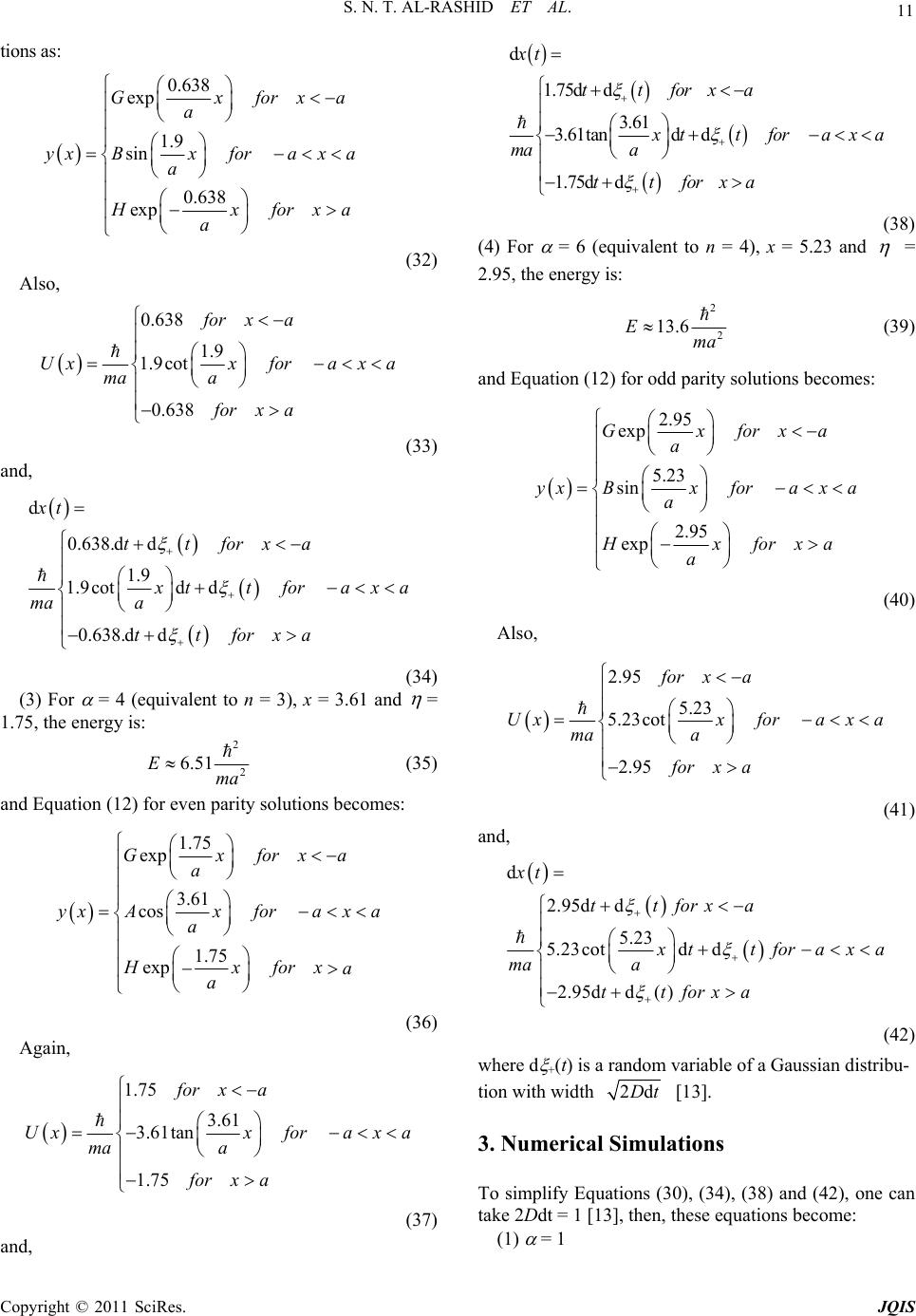

S. N. T. AL-RASHID ET AL.
11
tions as:

0.638
exp
1.9
sin
0.638
exp
Gxforx
a
yxBxforaxa
a
a
H
xforxa
a
 
 












(32)
Also,

0.638
1.9
1.9cot
0.638
for xa
Uxxforaxa
ma a
for xa










(33)
and,




d
0.638.dd
1.9
1.9cotd d
0.638.d d
xt
ttforxa
x
ttforax
ma a
ttforxa














 

a
(34)
(3) For
 = 4 (equivalent to n = 3), x = 3.61 and

=
1.75, the energy is:
2
2
6.51Ema  (35)
and Equation (12) for even parity solutions becomes:

1.75
exp
3.61
cos
1.75
exp
Gxforxa
a
yxAxforax a
a
Hxforx
a
 
 







 

a

(36)
Again,

1.75
3.61
3.61tan
1.75
for xa
Uxxforax a
ma a
for xa



 






(37)
and,





d
1.75d d
3.61
3.61tand d
1.75d d
xt
ttforxa
x
ttforax
ma a
ttforxa









 a





 


(38)
(4) For
 = 6 (equivalent to n = 4), x = 5.23 and

=
2.95, the energy is:
2
2
13.6Ema  (39)
and Equation (12) for odd parity solutions becomes:

2.95
exp
5.23
sin
2.95
exp
Gxforxa
a
yxBxforax a
a
Hxforx
a
 




a






 


(40)
Also,

2.95
5.23
5.23cot
2.95
for xa
Uxxforax a
ma a
for xa











(41)
and,




d
2.95d d
5.23
5.23cotd d
2.95dd( )
xt
ttforxa
x
ttforax
ma a
ttforxa














 

a
(42)
where d

+(t) is a random variable of a Gaussian distribu-
tion with width 2dDt [13].
3. Numerical Simulations
To simplify Equations (30), (34), (38) and (42), one can
take 2Ddt = 1 [13], then, these equations become:
(1)  = 1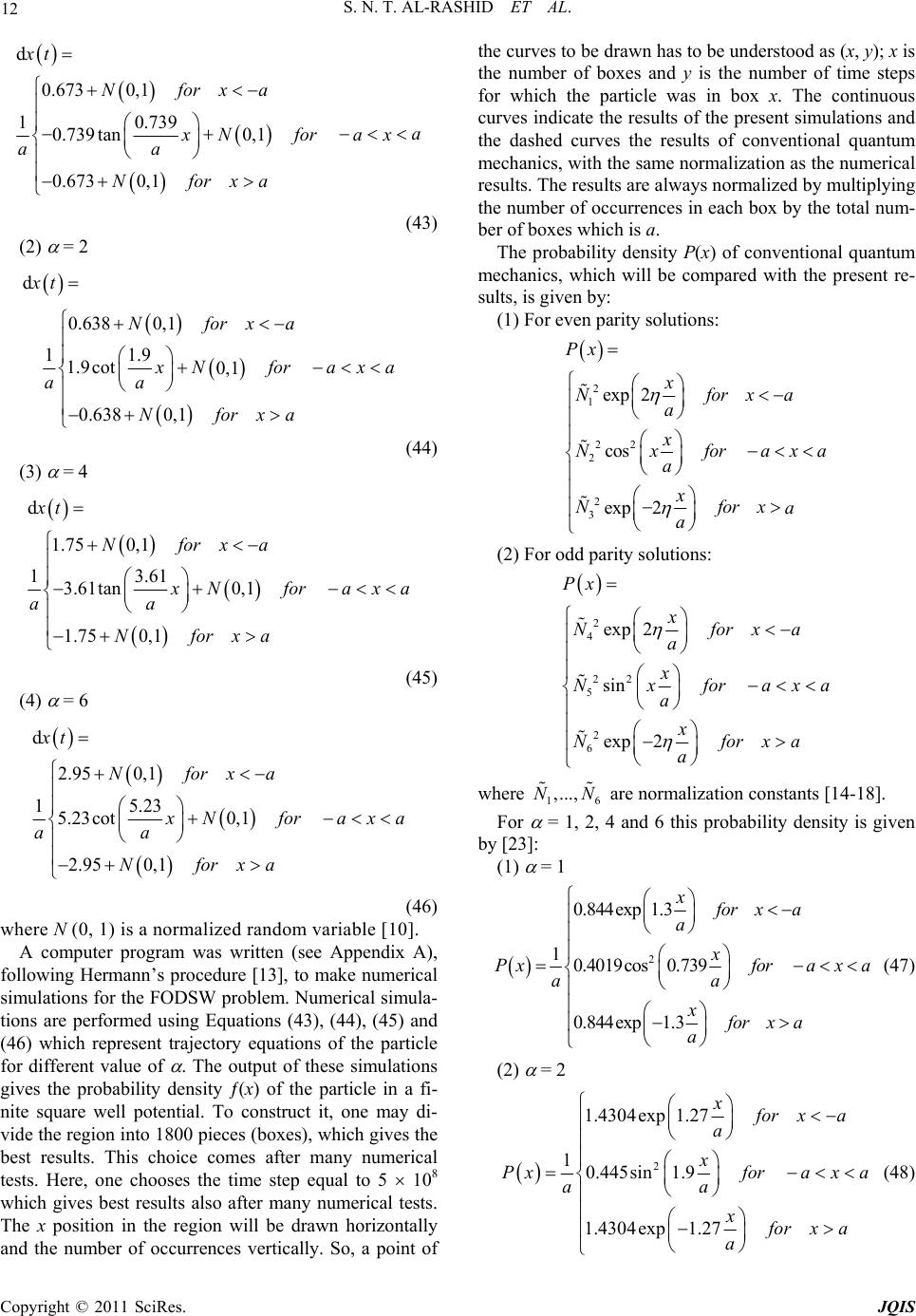

12 S. N. T. AL-RASHID ET AL.




d
0.673 0,1
10.739
0.739tan0,1
0.6730,1
xt
Nforxa
x
Nforax
aa
Nforxa








 

a
(43)
(2)  = 2

d
x
t



0.638 0,1
11.9
1.9cot 0, 1
0.6380,1
Nforxa
x
Nforax
aa
Nforxa







 

a
(44)
(3)  = 4




d
1.75 0,1
13.61
3.61tan 0,1
1.75 0,1
xt
Nforxa
x
Nforax
aa
Nforxa








 

a
(45)
(4)  = 6




d
2.95 0,1
15.23
5.23cot 0,1
2.95 0,1
xt
Nforxa
x
Nforax
aa
Nforxa








 

a
(46)
where N (0, 1) is a normalized random variable [10].
A computer program was written (see Appendix A),
following Hermann’s procedure [13], to make numerical
simulations for the FODSW problem. Numerical simula-
tions are performed using Equations (43), (44), (45) and
(46) which represent trajectory equations of the particle
for different value of  . The output of these simulations
gives the probability density ƒ(x) of the particle in a fi-
nite square well potential. To construct it, one may di-
vide the region into 1800 pieces (boxes), which gives the
best results. This choice comes after many numerical
tests. Here, one chooses the time step equal to 5  108
which gives best results also after many numerical tests.
The x position in the region will be drawn horizontally
and the number of occurrences vertically. So, a point of
the curves to be drawn has to be understood as (x, y); x is
the number of boxes and y is the number of time steps
for which the particle was in box x. The continuous
curves indicate the results of the present simulations and
the dashed curves the results of conventional quantum
mechanics, with the same normalization as the numerical
results. The results are always normalized by multiplying
the number of occurrences in each box by the total num-
ber of boxes which is a.
The probability density P(x) of conventional quantum
mechanics, which will be compared with the present re-
sults, is given by:
(1) For even parity solutions:


2
1
22
2
2
3
exp 2
cos
exp 2
Px
x
Nforx
a
x
Nxforax
a
x
Nforx
a



 
 

 











a
a
a
(2) For odd parity solutions:


2
4
22
5
2
6
exp 2
sin
exp 2
Px
x
Nforx
a
x
Nxforax
a
x
Nforx
a



 



 











a
a
a
6
where are normalization constants [14-18].
1
,...,NN

For  = 1, 2, 4 and 6 this probability density is given
by [23]:
(1)
 = 1

2
0.844exp 1.3
10.4019cos 0.739
0.844exp 1.3
xfor xa
a
x
Pxfora x a
aa
xfor x a
a
 














(47)
(2)  = 2

2
1.4304exp 1.27
10.445sin 1.9
1.4304exp 1.27
x
f
or xa
a
x
Pxforax a
aa
x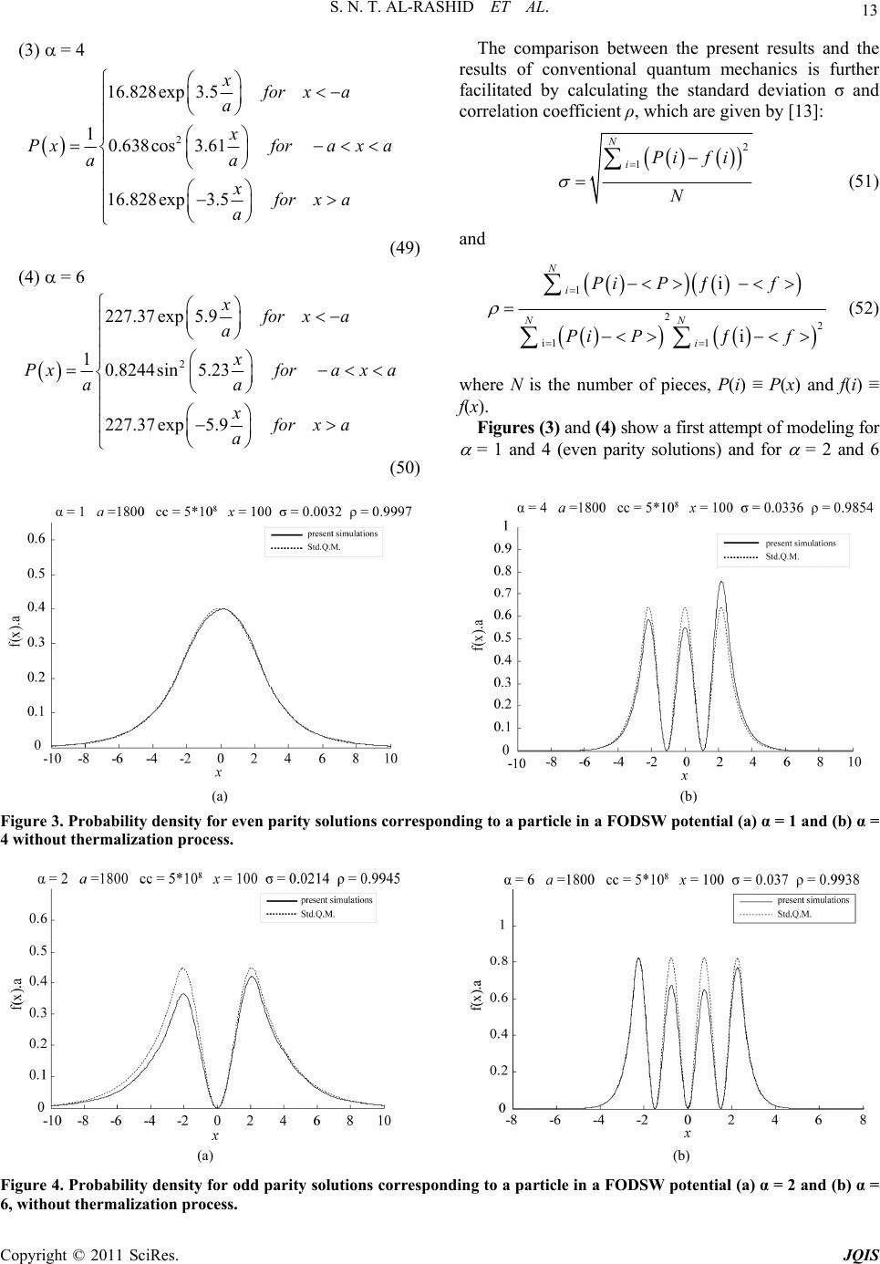
f
or xa
a
 














(48)

S. N. T. AL-RASHID ET AL.
13
(3)  = 4

2
16.828exp 3.5
10.638cos 3.61
16.828exp 3.5
xfor xa
a
x
Pxforax a
aa
xfor xa
a














The comparison between the present results and the
results of conventional quantum mechanics is further
facilitated by calculating the standard deviation σ and
correlation coefficient ρ, which are given by [13]:

 

2
1
N
iPif i
N


 (51)
and
(49)
(4)  = 6

2
227.37exp5.9
10.8244sin 5.23
227.37exp5.9
xfor xa
a
x
Pxforax a
aa
xfor xa
a
 
 







   
1
22
i1 1
ƒi
ƒi
N
i
NN
i
Pi Pf
Pi Pf



  


 


(52)









 where N is the number of pieces, P(i) ≡ P(x) and f(i) ≡
f(x).
Figures (3) and (4) show a first attempt of modeling for
 = 1 and 4 (even parity solutions) and for  = 2 and 6
(50)
(a) (b)
Figure 3. Probability density for even parity solutions corresponding to a particle in a FODSW potential (a) α = 1 and (b) α =
4 without thermalization process.
(a) (b)
Figure 4. Probability density for odd parity solutions corresponding to a particle in a FODSW potential (a) α = 2 and (b) α =
6, without thermalization process.

14 S. N. T. AL-RASHID ET AL.
Figure 5. Probability density for α = 6 (odd parity solution
corresponding to a particle in a FODSW potential after
y. The numerical simula-
present work that the behavior of a
Prof. Dr. L. Nottale (Di-
Paris, France) for clarifying
theory of scale relativity and
The Theory of Scale Relativity,” Interna-
of Modern Physics A, Vol. 7, No. 20,
-4936. doi:10.1142/S0217751X92002222
)
increasing the number of boxes.
(odd parity solutions) respectivel
tions start with arbitrary point which is x = 100 (corre-
sponding to box No. 100). In these figures, there is a clear
difference between the present results and the results of
quantum mechanics, that is measured by  and ρ.
Hermann [13] indicated in his work that the simula-
tions were restarted after 105 steps, or more, with a new
starting position. Then, better thermalization of the sys-
tem is obtained and convergence is increased. Tests in
the present work indicated that the thermalization proc-
ess as used by Hermann [13] cannot be applied here
without fixing additional parameters. This required very
long computer time and, therefore, was not adopted in
the present work. However, these tests also indicated that
the present results can be improved by increasing the
number of divisions of a (i.e., number of boxes). Figure
(5) shows the results obtained for
 = 6 after increasing
the number of boxes from 1800 to 2200.
4. Conclusions
It can be seen from the
quantum particle in an infinite one-dimensional square well
potential can be obtained without explicitly writing the
Schrödinger equation or using any conventional quantum
axiom. This leads one to conclude from the present work
that ScR is a well-founded theory for deriving quantum
mechanics from the concept of fractal space-time.
Even though many of the aspects of Hermann’s work
were used in the present work as they are, the application
of his approach to the present quantum mechanical prob-
lem was not a direct one. Successful applications were
not achievable without, among other things, a new ad-
justment for the time step dt after some deeper under-
standing of the underlying particle motion in the present
problem. It is expected that this understanding is neces-
mechanical problems along the lines of Hermann’s work
[13] and the present work. It is also concluded from the
attempts made in the present work to improve the results
of numerical simulation by parameter optimization, that
such attempts are successful in achieving some im-
provement, and that further improvement is possible, but
requires more computer time.
5. Acknowledgments
e would like to deeply thank
sary when attempts are made to solve other quantum
W
rector of Research, CNRS,
ome points regarding his s
for supplying some literature and Dr. R. Hermann
(Dept. of Physics, Univ. de Liege, Belgium) for his sug-
gestions concerning further applications of the theory of
scale relativity.
6. References
] L. Nottale, “[1
tional Journal
1992, pp. 4899
] L. Nottale, “Fractal Space-Time and Microphy[2 sics: To-
wards a Theory of Scale Relativity,” World Scientific,
Singapore, 1998.
[3] L. Nottale, “The Scale Relativity Program,” Chaos, Soli-
tons and Fractals, Vol. 10, No. 2-3, 1994, pp. 459-468.
doi:10.1016/S0960-0779(98)00195-7
[4] L. Nottale, “Scal
App
e Relativity and Fractal Space-Time:
,
779(96)00002-1
lication to Quantum Physics, Cosmology and Chaotic
Systems,” Chaos, Solitons and Fractals, Vol. 7, No. 6
1996, pp. 877-938. doi:10.1016/0960-0
[5] L. Nottale, “Scale Relativity, Fractal Space-Time and
Quantum Mechanics,” Chaos, Solitons and Fractals, Vol.
4, No. 3, 1994, pp. 361-388.
doi:10.1016/0960-0779(94)90051-5
[6] L. Nottale, “Scale Relativity, Fractal Space-Time and
Morphogenesis of Structures”, Sciences of the Interface,
Proceedings of International Symposium in Honor of O.
Rossler, ZKM Karlsruhe, 2000, p. 38.
[7] L. Nottale, “Scale Relativity,” Reprinted from “Scale In-
variance and Beyond,” In: B. Dubralle, F. Graner and D.
Sornette, Eds., Proceedings of Les Houches, EDP Sci-
ence, 1997, pp. 249-261.
[8] L. Nottale, “Scale Relativity and Quantization of the Uni-
verse-I, Theoretical Framework,” Astronomy and Astro-
physics, Vol. 327, No. 3, 1997, pp. 867-889.
[9] L. Nottale, G. Schumacher and J. Gray, “Scale Relativity
and Quantization of the Solar System,” Astronomy and
Astrophysics, Vol. 322, No. 3, 1997, pp. 1018-1025.
[10] L. Nottale and M. N. Célérier, “Derivation of the Postulates
of Quantum Mechanics from the First Principles of Scale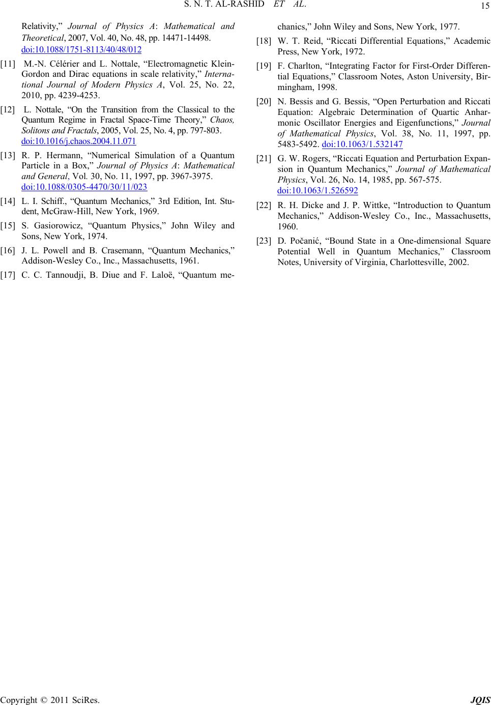

S. N. T. AL-RASHID ET AL.
15
Relativity,” Journal of Physics A: Mathematical and
Theoretical, 2007, Vol. 40, No. 48, pp. 14471-14498.
doi:10.1088/1751-8113/40/48/012
[11] M.-N. Célérier and L. Nottale, “Electromagnetic Klein-
Gordon and Dirac equations in scale relativity,” Interna-
tional Journal of Modern Physics A, Vol. 25, No. 22,
2010, pp. 4239-4253.
[12] om the Classical to the L. Nottale, “On the Transition fr
Quantum Regime in Fractal Space-Time Theory,” Chaos,
Solitons and Fractals, 2005, Vol. 25, No. 4, pp. 797-803.
doi:10.1016/j.chaos.2004.11.071
[13] R. P. Hermann, “Numerical Simulation of a Quantum
Particle in a Box,” Journal of Physics A: Mathematical
and General, Vol. 30, No. 11, 1997, pp. 3967-3975.
doi:10.1088/0305-4470/30/11/023
[14] cs,” 3rd Edition, Int.
[16] Quantum Mechanics
oё, “Quantum me-
[18] cademic
[19] fferen-
L. I. Schiff., “Quantum Mechani Stu-
dent, McGraw-Hill, New York, 1969.
[15] S. Gasiorowicz, “Quantum Physics,” John Wiley and
Sons, New York, 1974.
Addi J. L. Powell and B. Crasemann, “,”
son-Wesley Co., Inc., Massachusetts, 1961.
[17] C. C. Tannoudji, B. Diue and F. Lal
chanics,” John Wiley and Sons, New York, 1977.
W. T. Reid, “Riccati Differential Equations,” A
Press, New York, 1972.
F. Charlton, “Integrating Factor for First-Order Di
tial Equations,” Classroom Notes, Aston University, Bir-
mingham, 1998.
[20] N. Bessis and G. Bessis, “Open Perturbation and Riccati
Equation: Algebraic Determination of Quartic Anhar-
monic Oscillator Energies and Eigenfunctions,” Journal
of Mathematical Physics, Vol. 38, No. 11, 1997, pp.
5483-5492. doi:10.1063/1.532147
[21] G. W. Rogers, “Riccati Equation and Perturbation Expan-
sion in Quantum Mechanics,” Journal of Mathematical
Physics, Vol. 26, No. 14, 1985, pp. 567-575.
doi:10.1063/1.526592
[22] R. H. Dicke and J. P. Wittke, “Introduction to Quantum
Mechanics,” Addison-Wesley Co., Inc., Massachusetts,
1960.
[23] D. Počanić, “Bound State in a One-dimensional Square
Potential Well in Quantum Mechanics,” Classroom
Notes, University of Virginia, Charlottesville, 2002.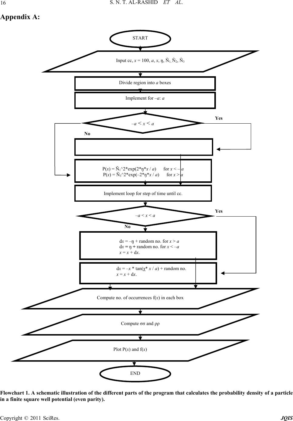

S. N. T. AL-RASHID ET AL.
16
ppendix A:
lowchart 1. A schematic illustration of the different parts of the program that calculates the probability density of a particle
square well potential (even parity).
A
F
in a finite
Implement for –a: a
START
Input cc, x = 100, a, x, ŋ, Ñ1, Ñ2, Ñ3
Divide region into a boxes
–a < x < a
P(x) = Ñ1^2*exp(2*ŋ*x / a) for x < – a
P(x) = Ñ3^2*exp(–2*ŋ*x / a) for x > a
Implement loop for step of time until cc.
–a < x < a
dx + random no. for x > a
dx = ŋ + random no. for x < –a
= –ŋ
x = x + dx.
dχ* x / a) + random no.
x = x + dx.
x = –x * tan(
Compute no. of occurrences f(x) in each box
Compute σσ and ρρ
Yes
Yes
No
No
Plot P(x)andf(x)
END

S. N. T. AL-RASHID ET AL.
17
Flowchart 2. A schematic illustration of the different parts ofrogram that calculates the probability density of a particle
a finite square well potential (odd parity).
Input cc, x = 100, a, χ, ŋ, Ñ4, Ñ5, Ñ6
Divide region into aboxes
Yes
Yes
No
No
Implement for –a: a
START
a< < a
x
–
P(x) = Ñ* x / a)
5^2*sin^2(χ
P(x) = Ñ4^2*e
P(x) = Ñ6^2*exp(–2*ŋ*x /a) for x > a hi how r u
xp(2*ŋ* x / a) for x < –a
Implement loop for step of time until cc.
–a< x< a
dx = –ŋ + rr x > a;
dx= ndom no. for x < –a;
x = x.
andom no. fo
ŋ + ra
+ dx
dx = –x *cot(x *x/a) + random no.
x = x + dx.
Comrences f(x) in each boxpute no. of occur
Compute σσ and ρρ
Plot P(x) and f(x)
END
the p
in
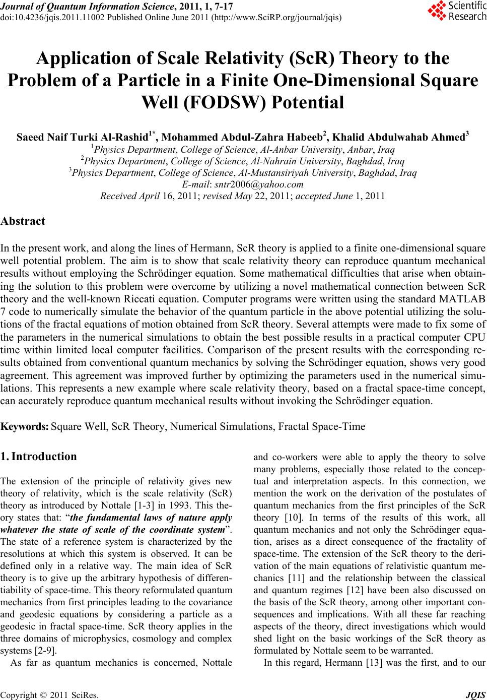