Applied Mathematics, 2011, 2, 783-790
doi:10.4236/am.2011.26105 Published Online June 2011 (http://www.SciRP.org/journal/am)
The Selection of Proper Auxiliary Parameters in the
Homotopy Analysis Method. A Case Study: Uniform
Solutions of Undamped Duffing Equation
Mustafa Turkyilmazoglu
Mathematics Department, University of Hacettepe, An kara, Turkey
Received March 20, 2011; revised May 9, 2011; accepted May 12, 2011
Abstract
The present paper is concerned with two novel approximate analytic solutions of the undamped Duffing
equation. Instead of the traditional perturbation or asymptotic methods, a homotopy technique is employed,
which does not require a small perturbation parameter or a large parameter for an asymptotic expansion. It is
shown that proper choices of an auxiliary linear operator and also an initial approximation during the imple-
mentation of the homotopy analysis method can yield uniformly valid and accurate solutions. The obtained
explicit analytical expressions for the solution predict the displacement, frequency and period of the oscilla-
tions much more accurate than the previously known asymptotic or perturbation formulas.
Keywords: Homotopy Analysis Method, Auxiliary Linear Operator, Initial Approximation, Duffing
Oscillator, Uniform Solution
1. Introduction
The importance of nonlinear Duffing equation has been
widely understood among the scientists since it plays a
key role in some important practical phenomena such as
periodic orbit extraction, non uniformity caused by an
infinite domain, nonlinear mechanical oscillators, predic-
tion of diseases, and so on.
Since the Duffing equation engulfs a strong nonli-
nearity within itself, it’s full analytical solution has not
been achieved so far. Therefore, considerable attention
has been directed towards the study of strongly nonlinear
oscillators and several methods have been used to find
approximate solutions to nonlinear oscillators. Most of
the methodologies involve the introduction of a small
parameter into the equation, which might be artificial,
and then expansion of the solution through the per-
turbation series around this parameter. However, the
solutions obtained within this approach may not be
uniform, restricting the applicability of such perturbation
methods [1,2]. To overcome the limitations of the
perturbative techniques, many novel techniques have
been proposed in recent years. For example, modified
Lindstedt-Poincare method [3,4] and variational iteration
methods [5]. Some other numerical and approximate
methods follow [6-10].
Liao in [11] proposed a new technique which is based
on the homotopy concept in topology, named the ho-
motopy analysis method (HAM). Unlike the aforemen-
tioned traditional perturbation methods, this technique
does not require a small perturbation parameter in the
equation. In this method, according to the homotopy
technique, a homotopy with an imbedding parameter is
constructed, and the imbedding parameter is considered
as a small parameter. Thus the original nonlinear pro-
blem is converted into an infinite number of linear
problems without using the perturbation techniques, see
the book by Liao [12]. Different from other methods, the
HAM provides a simple way to control and adjust the
convergence region of solution series by means of an
auxiliary parameter [13,14].
Following the introduction of HAM by Liao, He in [15]
proposed the so-called homotopy perturbation method
(HPM). Unfortunately, Sajid and Hayat [16] pointed out
that the so-called homotopy perturbation method has
nothing new except its new name, because the HPM is
only a special case of the homotopy analysis method
(HAM) when so that all results given by the HPM can be
obtained by the HAM as a special case. Moreover, as a
special case of the HAM, the HPM can not give con-

M. TURKYILMAZOGLU 784
vergent series solution for strongly nonlinear problems.
Abbasbandy in [17] gave a simple example to show that,
like perturbation approximations, the results given by the
HPM are divergent when the physical parameters
become large. Among many other authors VanGorder
and Vajravelu in [18] also pointed out this fact. More
recently, Liang and Jeffrey in [19] pointed out that in
some cases the series solution given by the HPM and
VIM (another method proposed also by He in [20]) is
divergent at all points except that however de-
fines the initial condition.
=0t
We in the present paper use the homotopy analysis
technique for the solution of the nonlinear Duffing
equation. Better auxiliary linear operators and initial
approximations are the essential target to be used here
within the homotopy concept so that highly accurate
solutions have been obtained. The proposed linear
operators together with the homotopy analysis method
provide formulas for the displacement, frequency and
period of the oscillations, which are valid for all the
existing parameters and also are more accurate than
those already available in the literature.
The following strategy is adopted in the rest of the
paper. In Section 2 the idea of homotopy analysis
method is laid out. Application of the method is
implemented in Section 3, in which, first the homotopy
analysis method is revisited and later using different
auxiliary parameters and initial approximations, analytic
expressions are derived yielding better results. Section4
presents compari- sons of the period and displacement
between those in [15], our findings and the exact
numerical ones. Finally conclusions follow in Section 5.
2. The Homotopy Analysis Method
Liao in [1] proposed a new kind of analytic technique for
nonlinear problems, namely the homotopy analysis
method. This method is based on the homotopy and has
several advantages. To underline, firstly its validity does
not depend upon whether or not nonlinear equations
under consideration contain small or large parameters,
hence it can solve more of strongly nonlinear equations
than the perturbation techniques. Secondly, it provides us
with a great freedom to select proper auxiliary linear
operators and initial guesses so that uniformly valid
approximations can be obtained. Thirdly, it gives a
family of approximations which are convergent in a
larger region. Liao successfully applied the homotopy
analysis method to solve some nonlinear problems in
mechanics. For example, Liao in [21] gave a purely
analytic solution of 2D Blasius’s viscous flow over a
semi-infinite flat plate, which is uniformly valid in the
whole physical region. Further examples are provided
within the reference [12]. To briefly describe the method
let’s consider the following nonlinear differential equa-
tion




=0, Nu frr

 (1)
with boundary conditions
,=0,
u
Bu r
n

 


 (2)
where is a nonlinear operator, is a boundary
operator, is an unknown analytic function and
NuB

is
the boundary of the domain . By this technique, we
construct a homotopy



,vrp from the cartesian set


0, 1 to which satisfies R





  
0
,=1 =0HvppLvuphNufr  

,(3)
where [0,1]

p is an embedding parameter, 0 is an
initial approximation of Equation (1) that satisfies the
boundary condition (2) and is a constant that can be
adjusted to speed the convergence. It is clear from
Equation (3) that for and respectively the
followings hold
u
h
=0p1=p




 
0
,0== 0,
,1== 0.
HvLv u
HvNu fr

 (4)
Hence, it can be deduced from (4) that the deformation
process of from zero to unity is just that of the
solution from
p


0
ur to . Further, considering
as a parameter, the solution to system (1-2) can be
naturally expressed taking into account a Taylor
expansion of the solution at and later
imposing the expansion at

ur
,vt
=1p
p

p

,
=0p
 
0
=1
=
k
k
utu tut

 (5)
where are defined by
k
u
=0
1
=!
k
p
u
ukp

.
3. Application to Duffing Equation
Duffing equation describes many kinds of nonlinear
oscillatory systems in physics, mechanics and engi-
neering. The unforced, undamped Duffing equation that
we consider consists of the nonlinear initial value system
 
2
3
2
d=0, 0=, 0=0.
d
uuuu Au
t


 (6)
The parameters

and
A
in (6) measure respec-
tively the nonlinearity and amplitude of the displacement


ut. Actually the period of the solution can be for-
mulated analytically as in [2]

2 π
2
2 0
22
4d
=, =.
21
11sin
xA
Tk
A
Akx





 (7)

M. TURKYILMAZOGLU785
For the system (6) Liao in [22] suggested the
subsequent auxiliary linear operator

2
2
d
=d
u
Lu u
t

(8)
with an assumption of the initial solution of the form
0=cos,uA t

(9)
such that




is a nonzero unknown constant with the
property of . Considering the homotopy in-
troduced in (3) with and imposing the constraint
that no secular terms are allowed, He in [15] obtained a
first-order approximation to the solution in subsequent
form

0=1
h=1
 
23
22
3
=cos cos
41 491
AA
ut

3, t





(10)
in which

is defined as
22
10764 10449
=.
18
24
A
AA 

  
(11)
It should be remarked here that the solution given in
(10) has a non removable singularity for =1

.
Carrying out a further step, it is easy to obtain the
next-order solution 2 in (5) which can later be com-
bined with (10) to form a second-order solution. He then
obtained the period of the approximate solution by
u
2π
=T,

(12)
with

given as in (11). He, later claimed that the
solution he achieved by the homotopy technique with the
properly chosen auxiliary parameters is of high accuracy
and it is valid for a very large values of

. Denoting the
ratio of exact period (7) to approximate one (12) in the
limit of

tending to infinity as ra
t
, He found that
(it should be emphasized that a simple
error occurred in [15] for the evaluation of
= 96rat 1.040 ra
t
).
Therefore, He in [15] concluded that for any value of

the maximal relative error is only 4 percent.
In place of the linear operator (8), He [23] proposed to
use

2
2
2
d
=d
u
Lu u
t

 (13)
with the same assumption of the initial solution as in (9)
and . If the occurrence of secular terms in the
solution is eliminated in the first iteration, the solution to
Duffing Equation (6) can be written at the first-order in
the form
1=h
3
2
sinsin 2
=cos ,
16
A
t
uA tt


  (14)
with

defined as
2
1
=43
2.
A

  (15)
It can be immediately seen that the displacement
in (14) does not blow up for any physical value of
u

and the form of

obtained in (15) is much simpler
than Equation (11) obtained in [15]. With this frequency,
the ratio between the exact and approximate period can
be computed as 1.0222 in the limit

. Thus (15)
represents a better estimate and only 2 percent relative
error occurs, even for infinite value of

. A comparison
between (10-11) and (14-15) will be performed later in
section Section 4.
It is a well-known fact that in the homotopy method
there is a great freedom for the choice of auxiliary linear
operator and initial approximate solution. We prove, in
what follows, that with different proper selections, a
better solution than (10-11) can be obtained.
3.1. A New Proposed Homotopy 1
Making a substitution =t

 permits the frequency

to appear explicitly in the Duffing Equation (6). This is
actually a coupled technogy of homotopy analysis me-
thod with the Lindstedt Poincare method. Afterwards,
keeping the linear operator as in (8) with replaced by
t

, choosing the initial approximation as 0=cuAos

with 2
1
=h
A

(note that this selection of is nece- h
ssary to keep the consistency in the limit



). If the
occurrence of secular terms in the solution is eliminated
in the first iteration, the leading-order 0

is found to be
the same as (15) and the solution to the transformed
Duffing equation can be written at the first-order in the
form

1
=31coscos3
32
uA

.

  (16)
With the frequency 0 =

 , the ratio between the
exact and approximate is the same as for homotopy
approach of He [23] in the limit 

. To get a better
estimate and hence improve the frequency, we again set
the coefficient of

cos to disappear so that secular
terms in the next solution will be eliminated. This results
in
2
12
3
=
128 43
A
wA

,

 (17)
leading to
2
01 2
256 189
==
128 43
A
A

 



whose large

limit yields a ratio 1.00623, so only 0.62

M. TURKYILMAZOGLU 786
t
percentage relative error is observed, which is much
better than the above approaches.
3.2. A New Proposed Homotopy 2
If we now select the linear operator as in (13) but assume
the initial approximation to the solution as
0=cosuA

, with

denoting the frequency of the
solution different from that of linear solution

, they
can be determined at the first iteration by restricting the
appearance of secular terms at the next level. Within this
approach

and

are found to be



4 221/31/32/32/3
1/3
4096409633601323808 38083 1433043
= ,
12 3
iiiAA ii  


 
(18)
22
22
97 9
=,
1
A
A





where

24263
4224263 84
= 26214473113652809659833
6486327681239041665369251317113.
AAA
AAAA

A


 
  
By this means, the homotopy method (3) yields the first-order solution





 

222222222
4224
2 cos18131822cos2
=cos .
410 9
A
tA AA
uA t
 

 

t
(19)
The forms of the solution in (19) and of the frequency
in (18) are more complicated when compared with those
of (10-11) and (14-15). However, after a straightforward
evaluation it is found that in the limit = 0.997314rat

, resulting in only 0.26 percent maximal relative
error, which is best of all among those presented in [15]
and above by our two approaches.
4. Discussion of the Results
In this section, to show the advantages of our homotopy
approaches, a comparison is made between the full nu-
merical simulation results of (6), those of He in [15] and
the ones obtained in section Section 3. We particularly
choose the parameters =1
A
and =1

in what
follows. For these specific values, it is straightforward to
compute the correspondences of the periods, which are
tabulated in Table 1. As compared to the exact period,
our homotopy technique is seen to give extremely more
accurate results than the homotopy perturbation em-
ployed in [15].
We next present numerical simulation results of the
displacement function. Figure 1 shows the exact nume-
rical and second-order approximate solution of He, wher-
eas Figures 2-4 demonstrate the exact numerical and
first-order solutions from the homotopy approaches. It is
observed from Figure 1 related to the second-order
homotopy perturbation method of He that the uniformity
of the approximate solution gets weakened as in-
creases. On the other hand, our first-order approach in
the homotopy analysis gives extremely accurate solu-
tions when compared with the exact solution. Particu-
larly as seen from Figure 4, a much higher accuracy can
be observed from the approach 3. Thus, the analytic
approximations as displayed in Figures 2-4 are suffi-
ciently reliable and can be used in the analysis of Duff-
ing oscillator in further research.
t
It should be emphasized that only the first-order app-
roximate solutions that we obtained in Section 3 reveal
ex- cellent agreement with the exact numerical solutions.
Addition of higher approximations from the homotopy
technique would yield more remarkable agreement. It is
furthermore worthwhile to state that the homotopy solu-
tions obtained here are valid for all the values of the
parameters
A
and

. Therefore, we do not need to
approximate the small

perturbation solutions or the
large

asymptotic solutions as in [2]. In fact, our
Table 1. Illustrating the periods for the Duffing Equation (6)
for A = 1 and ε = 1. First is the exact, second is from He in
[15], third is from approach of He [23], fourth is from
approach 1 and the fifth is from approach 2. s
4.76802 4.73233 4.74964 4.78166 4.76877

M. TURKYILMAZOGLU 787
Figure 1. Solution of the Duffing Equation (6): straight curve from the numerical solution and dashed curve from the
second-order solution of He (10).
Figure 2. Solution of the Duffing Equation (6): straight curve from the numerical solution and dashed curve from the
first-order solution of approach of He [23] (14).

M. TURKYILMAZOGLU 788
Figure 3. Solution of the Duffing Equation (6): straight curve from the numerical solution and dashed curve from the
first-order solution of approach 1 (16).
Figure 4. Solution of the Duffing Equation (6): straight curve from the numerical solution and dashed curve from the
first-order solution of approach 2 (19).

M. TURKYILMAZOGLU 789
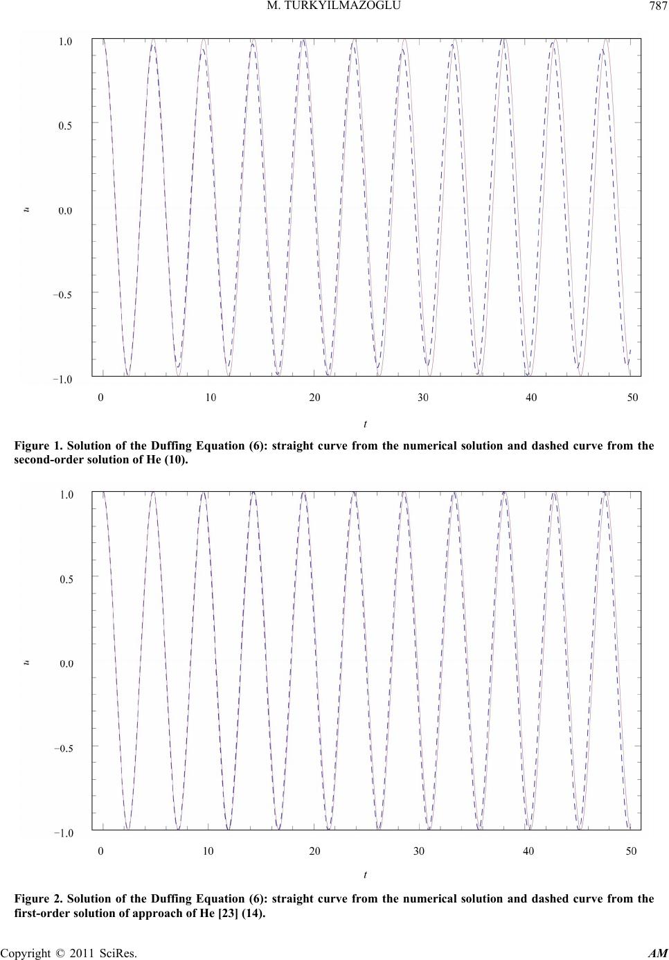
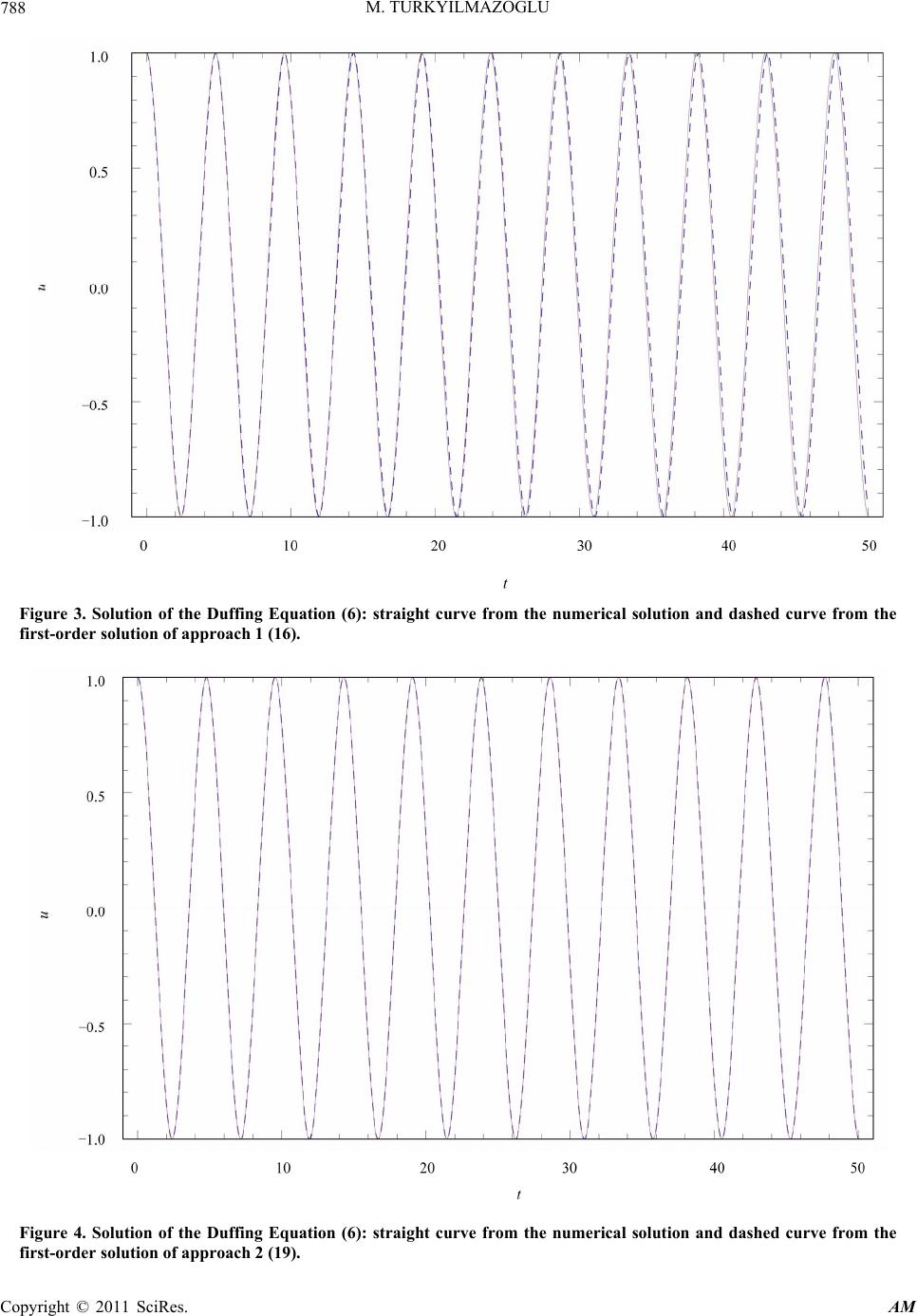
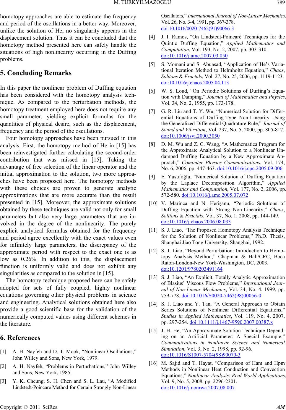
homotopy approaches are able to estimate the frequency
and period of the oscillations in a better way. Moreover,
unlike the solution of He, no singularity appears in the
displacement solution. Thus it can be concluded that the
homotopy method presented here can safely handle the
situations of high nonlinearity occurring in the Duffing
problems.
5. Concluding Remarks
In this paper the nonlinear problem of Duffing equation
has been considered with the homotopy analysis tech-
nique. As compared to the perturbation methods, the
homotopy treatment employed here does not require any
small parameter, yielding explicit formulas for the
quantities of physical desire, such as the displacement,
frequency and the period of the oscillations.
Four homotopy approaches have been pursued in this
analysis. First, the homotopy method of He in [15] has
been reinvestigated further calculating the second-order
contribution that was missed in [15]. Taking the
advantage of free selection of the linear operator and the
initial approximation to the solution, two more approa-
ches have been proposed here. The homotopy methods
with these choices are proven to generate analytic
approximations that are more accurate than the result
presented in [15]. Moreover, the approximate solutions
obtained by these techniques are valid not only for small
parameters but also very large parameters that are in-
volved in the degree of the nonlinearity. The purely
explicit analytical formulas obtained for the frequency
and period agree excellently with the exact values even
for infinitely large parameters, the discrepancy of the
approximate period with respect to the exact one is as
low as 0.26%. In addition to this, the displacement
function is uniformly valid and does not exhibit any
singularities as compared to the solution in [15].
The homotopy technique proposed here can be safely
adopted for sets of fully coupled, highly nonlinear
equations governing other physical problems in science
and engineering. Analytical solutions obtained here also
provide a good scientific base for the validation of the
numerically computed values using different schemes in
the literature.
6. References
[1] A. H. Nayfeh and D. T. Mook, “Nonlinear Oscillations,”
John Willey and Sons, New York, 1979.
[2] A. H. Nayfeh, “Problems in Perturbations,” John Willey
and Sons, New York, 1985.
[3] Y. K. Cheung, S. H. Chen and S. L. Lau, “A Modified
Lindstedt-Poincaré Method for Certain Strongly Non-Linear
Oscillators,” International Journal of Non-Linear Mechanics,
Vol. 26, No. 3-4, 1991, pp. 367-378.
doi:10.1016/0020-7462(91)90066-3
[4] J. I. Ramos, “On Lindstedt-Poincaré Techniques for the
Quintic Duffing Equation,” Applied Mathematics and
Computation, Vol. 193, No. 2, 2007, pp. 303-310.
doi:10.1016/j.amc.2007.03.050
[5] S. Momani and S. Abuasad, “Application of He’s Varia-
tional Iteration Method to Helmholtz Equation,” Chaos,
Solitons & Fractals, Vol. 27, No. 25, 2006, pp. 1119-1123.
doi:10.1016/j.chaos.2005.04.113
[6] W. S. Loud, “On Periodic Solutions of Duffing’s Equa-
tion with Damping,” Journal of Mathematics and Physics,
Vol. 34, No. 2, 1955, pp. 173-178.
[7] G. R. Liu and T. Y. Wu, “Numerical Solution for Differ-
ential Equations of Duffing-Type Non-Linearity Using
the Generalized Differential Quadrature Rule,” Journal of
Sound and Vibration, Vol. 237, No. 5, 2000, pp. 805-817.
doi:10.1006/jsvi.2000.3050
[8] D. M. Wu and Z. C. Wang, “A Mathematica Program for
the Approximate Analytical Solution to a Nonlinear Un-
damped Duffing Equation by a New Approximate Ap-
proach,” Computer Physics Communications, Vol. 174,
No. 6, 2006, pp. 447-463. doi:10.1016/j.cpc.2005.09.006
[9] E. Yusufoğlu, “Numerical Solution of Duffing Equation
by the Laplace Decomposition Algorithm,” Applied
Mathematics and Computation, Vol. 177, No. 2, 2006, pp.
572-580. doi:10.1016/j.amc.2005.07.072
[10] V. Marinca and N. Herişanu, “Periodic Solutions of
Duffing Equation with Strong Non-Linearity,” Chaos,
Solitons & Fractals, Vol. 37, No. 1, 2008, pp. 144-149.
doi:10.1016/j.chaos.2006.08.033
[11] S. J. Liao, “The Proposed Homotopy Analysis Technique
for the Solution of Nonlinear Problems,” Ph.D. Thesis,
Shanghai Jiao Tong University, Shanghai, 1992.
[12] S. J. Liao, “Beyond Perturbation: Introduction to Homo-
topy Analysis Method,” Chapman & Hall/CRC, Boca
Raton-London-New York-Washington, DC, 2003.
doi:10.1201/9780203491164
[13] S. J. Liao, “An Explicit, Totally Analytic Approximation
of Blasius’ Viscous Flow Problems,” International Jour-
nal of Non-Linear Mechanics, Vol. 34, No. 4, 1999, pp.
759-778. doi:10.1016/S0020-7462(98)00056-0
[14] S. J. Liao and Y. Tan, “A General Approach to Obtain
Series Solutions of Nonlinear Differential Equations,”
Studies in Applied Mathematics, Vol. 119, No. 4, 2007,
pp. 297-254. doi:10.1111/j.1467-9590.2007.00387.x
[15] J. H. He, “An Approximate Solution Technique Depend-
ing on an Artificial Parameter: A Special Example,”
Communications in Nonlinear Science and Numerical
Simulation, Vol. 3, No. 2, 1998, pp. 92-96.
doi:10.1016/S1007-5704(98)90070-3
[16] M. Sajid and T. Hayat, “Comparison of Ham and Hpm
Methods in Nonlinear Heat Conduction and Convection
Equations,” Nonlinear Analysis: Real World Applications,
Vol. 9, No. 5, 2008, pp. 2296-2301.
doi:10.1016/j.nonrwa.2007.08.007

M. TURKYILMAZOGLU 790
[17] S. Abbasbandy, “The Application of the Homotopy Ana-
lysis Method to Nonlinear Equations Arising in Heat
Transfer,” Physics Letter A, Vol. 360, No. 1, 2006, pp.
109-113. doi:10.1016/j.physleta.2006.07.065
[18] R. A. Van Gorder and K. Vajravelu, “Analytic and Nu-
merical Solutions to the Lane-Emden Equation,” Physics
letter A, Vol. 372, No. 39, 2008, pp. 6060-6065.
doi:10.1016/j.physleta.2008.08.002
[19] S. Liang and D. J. Jeffrey, “Comparison of Homotopy
Analysis Method and Homotopy Perturbation Method
through an Evolution Equation,” Communications in
Nonlinear Science and Numerical Simulation, Vol. 14,
No. 12, 2009, pp. 4057-4064.
doi:10.1016/j.cnsns.2009.02.016
[20] J. H. He, “Variational Iteration Method—Some Recent
Results and New Interpretations,” Journal of Computa-
tional and Applied Mathematics, Vol. 207, No. 1, 2007,
pp. 3-17. doi:10.1016/j.cam.2006.07.009
[21] S. J. Liao, “A Uniformly Valid Analytic Solution of
Two-Dimensional Viscous Flow over a Semi-Infinite Flat
Plate,” Journal of Fluid Mechanics, Vol. 385, 1999, pp.
101-128.
[22] S. J. Liao and I. Pop, “Explicit Analytic Solution for
Similarity Boundary Layer Equations,” International
Journal of Heat and Mass Transfer, Vol. 47, No. 1, 2004,
pp. 75-85. doi:10.1016/S0017-9310(03)00405-8
[23] J. H. He, “Some Asymptotic Methods for Strongly
Nonlinear Equations,” International Journal of Modern
Physics B, Vol. 20, No. 10, 2006, pp. 1141-1199.
doi:10.1142/S0217979206033796