Applied Mathematics, 2011, 2, 699-704
doi:10.4236/am.2011.26092 Published Online June 2011 (http://www.SciRP.org/journal/am)
G-Contractive Sequential Composite Mapping Theorem in
Banach or Probabilistic Banach Space and Application to
Prey-Predator System and A & H Stock Prices
Tianquan Yun
Department of En gi ne eri n g Mechanics, School of Civil Engineering and Transportation,
South China University of Technology, Guangzhou, China
Received March 21, 201 1; revised April 7, 2011; accepted April 10, 2011
Abstract
Theorems of iteration g-contractive sequential composite mapping and periodic mapping in Banach or prob-
abilistic Bannach space are proved, which allow some contraction ratios of the sequence of mapping might
be larger than or equal to 1, and are more general than the Banach contraction mapping theorem. Application
to the proof of existence of solutions of cycling coupled nonlinear differential equations arising from
prey-predator system and A & H stock prices are given.
Keywords: G-Contractive Mapping, Periodic Mapping, Probabilistic Banach Space, Prey-Predator System,
Differential Equation of Stock Price
1. Introduction
Fixed point theorems play an important role for the proof
of existence of solution of equations of algebra, differen-
tial, and integral, etc. It has been applied to many areas
such as mathematical economics, game theory, dynamic
optimization, functional analysis, etc. A lot of research
work on fixed point theorems of various mappings on
different spaces have been done (see [1,2] and their ref-
erences). Among these works, the Banach contraction
mapping theorem is a basic theorem for many research
works. However, the Banach contraction mapping theo-
rem needs a serious restriction, that is, all contraction
mapping ratios must less than a constant less than 1. In-
stead of this restriction, a loosed restriction which allows
some contraction mapping ratios to be greater or equal to
1 but the geometric mean of contraction mapping ratios
of the sequential mapping (simplifying as “g-contraction
mapping”) must less than a constant less than 1, is pro-
posed by the author [2]. In this paper, the iterative
g-contraction mapping and periodic mapping theorems in
Banach or probabilistic Banach space are proved and
application to cycling coupled nonlinear differential
equations arising from prey-predator system and A & H
stock prices are given..
The A-stock market in mainland China is a new de-
veloping market and is going to connect the rule with
international market. The H-stock market in Hong Kong
is a district international stock market. Many companies
have their shares in both A- and H-markets, e.g., the
China Petrol (601857) and Petro China (HK0857), a sig-
nificant share in A-stock market. Although there are
some papers on computational stock price based on cer-
tain model [3,4], however, no paper on quantitative
analysis of stock prices on different stock markets has
been found. This paper establishes a cycling coupled
differential equations of stock prices of A & H shares,
and uses the theorem to prove the existence of solutions
and further more find the solution as well as the prey-
predator pro ble m.
2. Main Results
In the following, let us consider a sequential mapping


i
T,


1, 2,iN , 1, i
:
ii i
TX X


X
M , M
is a probability Banach space, i.e., a comp lete non empty
metric space satisfied probabilistic requirements.
Definition 2.1. A sequential mapping


i
T satisfied
(1) is called the sequential composite mapping.

11
: or
,
iiii ii
ii
TXXx Tx
xX MiN


 

,
(1)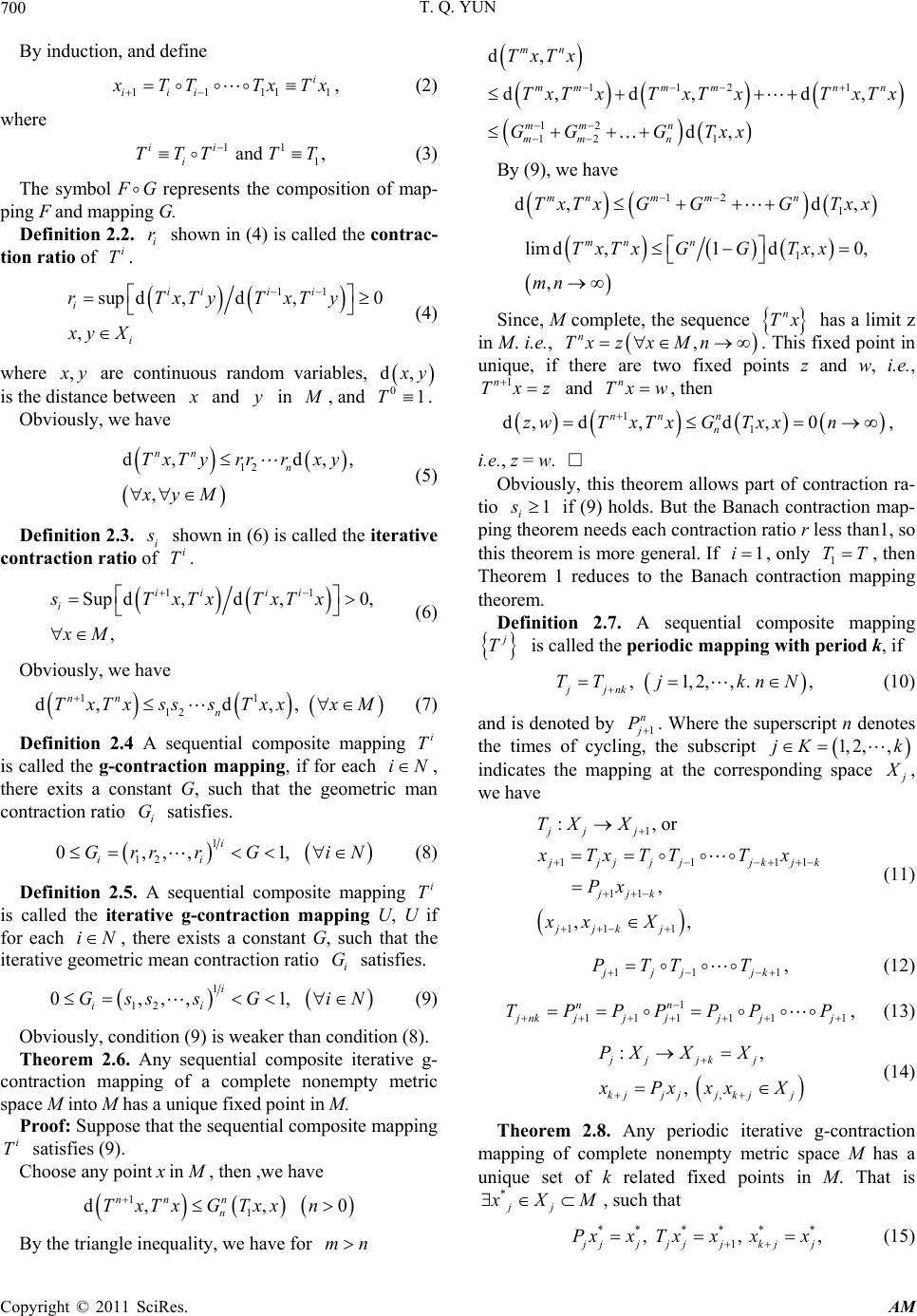

T. Q. YUN 700
1
By induction, and d efine
1111
i
iii
x
TTTx Tx

 

, (2)
where
11
1
and ,
ii
i
TTT TT

 (3)
The symbol F G represents the composition of map-
ping F and mapping G.

Definition 2.2. shown in (4) is called the contrac-
tion ratio of . i
r
i
T
 
11
sup d,d,0
,
iii i
i
i
rTxTyTxTy
xy X






(4)
where ,
x
y are continuous random variables,


d,
x
y
is the distance between
x
and in y
M
, and 01T

.
Obviously, we have



12
d, d,
,
nn n
TxTyrrrxy
xyM


,
(5)
Definition 2.3. i
s
shown in (6) is called the iterative
contraction ratio of .
i
T

11
Sup d,d,0,
,
ii ii
i
sTxTxTxTx
xM







(6)
Obviously, we have




11
12
d,d,,
nn n
TxTx sssTxxxM


 (7)
Definition 2.4 A sequential composite mapping
is called the g-contraction mapping, if for each
i
T
iN

,
there exits a constant G, such that the geometric man
contraction ratio satisfies.
i
G
 
1
12
0,,,1,
i
ii
Grr rGiN

(8)
Definition 2.5. A sequential composite mapping
is called the iterative g-contraction mapping U, U if
for each , there exists a constant G, such that the
iterative geometric mean contraction ratio satisfies.
i
T
iN
i
G
 
1
12
0,,,1,
i
ii
Gss sGiN

(9)
Obviously, condition (9) is weaker than condition (8).
Theorem 2.6. Any sequential composite iterative g-
contraction mapping of a complete nonempty metric
space M into M has a unique fixed point in M.
Proof: Suppose that the sequential composite mapping
satisfies (9).
i
TChoose any point
x
in M , then ,we have


 
11
d,,
nn n
n
TxTx GTxxn
0
By the triangle inequality, we have for
mn


 


112 1
12
12 1
d,
d,d,d ,
d,
mn
mmm mn n
mm n
mm n
TxTx
TxTx TxTxTxTx
GG GTxx
 


 




By (9), we have





12 1
d, d,
mnm mn
TxTx GGGTxx






1
limd,1d ,0,
,
mn n
TxTx GGTxx
mn





Since, M complete, the sequence has a limit z
in M. i.e.,

n
Tx



,
n
Txzx Mn

 
z
. This fixed point in
unique, if there are two fixed points z and w, i.e.,
1n
Tx


and n Txw

, then





11
d,d,d ,0
nn n
n
zwT xTxGTxxn



,
i.e., z = w. 
Obviously, this theorem allows part of contraction ra-
tio if (9) holds. But the Banach contraction map-
ping theorem needs each contraction ratio r less than1, so
this theorem is more general. If , only 1
1
i
s
1iTT

, then
Theorem 1 reduces to the Banach contraction mapping
theorem.
Definition 2.7. A sequential composite mapping


j
T is called the periodic mapping with period k, if


, 1,2,,. ,
jjnk
TT jknN

  (10)
and is denoted by 1
n
j
P

. Where the superscript n denotes
the times of cycling, the subscript


1, 2,,jKk 
indicates the mapping at the corresponding space
j
X
,
we have

1
11
11
11 1
:, or
,
,,
jjj
11
j
jjjjjkj k
jjk
jjk j
TXX
xTxTT Tx
Px
xx X




 




 
1
(11)
11
j
jj jk
PTT T



 , (12)
1
111 11
nn 1
j
nk jjjjjj
TP PPPPP


 
 



, (13)

,
:,
,
jjjk j
kjj jjkjj
PX XX
x
Pxx xX




(14)
Theorem 2.8. Any periodic iterative g-contraction
mapping of complete nonempty metric space M has a
unique set of k related fixed points in M. That is
*jj
x
XM, such that
******
1
, , ,
j
jjjjjkjj
Pxx Txxxx

  (15)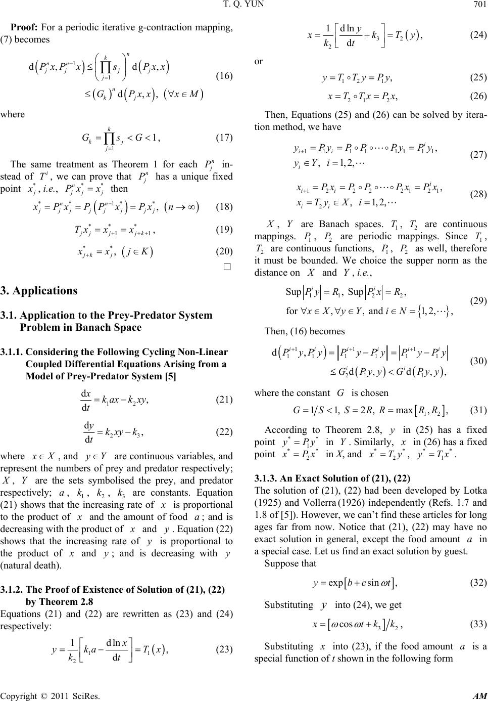

T. Q. YUN701

Proof: For a periodic iterative g-contraction mapping,
(7) becomes


  
1
1
d, d,
d,,
n
k
nn
jjj j
j
n
kj
PxPxsPxx
GPxxxM






 (16)
where
1
1
k
kj
j
GsG


, (17)
The same treatment as Theorem 1 for each n
j
P in-
stead of , we can prove that
i
Tn
j
P has a unique fixed
point *
j
x
, i.e., *n*
j
j
Px x
**nn
j

1
then


1 *
,
jj jjjj jj
xPxPPx Pxn

 
* (18)
** *
1
j
jj jk
Tx xx



, (19)


**
,
jk j
x
xjK
 (20)

3. Applications
3.1. Application to the Prey-Predator System
Problem in Banach Space
3.1.1. Considering the Following Cycling Non-Linear
Coupled Differential Equa tions Arisin g from a
Model of Prey-Predator System [5]
12
d,
d
xkax kxy
t (21)
2
d,
d
ykxyk
t
3
(22)
where
x
X, and
y
Y are continuous variables, and
represent the numbers of prey and predator respectively;
X
, are the sets symbolised the prey, and predator
respectively; , , , are constants. Equation
(21) shows that the increasing rate of
Ya1 2
kk 3 k
x
is proportional
to the product of
x
and the amount of food ; and is
decreasing with the produ ct of a
x
and . Equation (22)
shows that the increasing rate of is proportional to
the product of
y
y
x
and ; and is decreasing with
(natural death). y y
3.1.2. The Proof of Existence of Solution of (21), (22)
by Theorem 2.8
Equations (21) and (22) are rewritten as (23) and (24)
respectively:

1
2
1dln ,
d
x
ykaTx
kt





32
2
1dln ,
d
y
x
kTy
kt




(24)
or
12 1
,yTTyPy

 (25)
21 2
,
x
TTxPx

 (26)
Then, Equations (25) and (26) can be solved by itera-
tion method, we have
11 111111
,
, 1,2,
i
ii
i
yPyPP PyPy
yYi
 


 (27)
12 222121
2
,
, 1,2,
i
ii
ii
x
PxP PPxPx
xTyXi
 
 

 (28)
X
, are Banach spaces. 1, 2 are continuous
mappings. 1, 2 are periodic mappings. Since 1 T,
2 are continuous functions, 1, 2 as well, therefore
it must be bounded. We choice the supper norm as the
distance on
YT T
P P
TP P
X
and Y, i.e.,
 
11 22
Sup, Sup,
for ,, and 1,2,,
ii
Py RPxR
xXyYiN

 
(29)
Then, (16) becomes


 
11 1
11 1111
21 1
d,
d,d,,
ii iiii
ii
PyPyPyPy PyPy
GPyy G Pyy
 

 (30)
where the constant is chosen
G


12
11, 2, max,GS SRRRR , (31)
According to Theorem 2.8, in (25) has a fixed
point y
**
1
y
Py in Y. Similarly,
x
in (26) has a fixed
point *
2*
x
Px in X, and **
2
x
Ty, **
1
y
Tx.
3.1.3. An Exact Solution of (21), (22)
The solution of (21), (22) had been developed by Lotka
(1925) and Vollerra (1926) independently (Refs. 1.7 and
1.8 of [5 ]). How ev er, we can’t f ind th ese articles f or long
ages far from now. Notice that (21), (22) may have no
exact solution in general, except the food amount in
a special case. Let us find an exact solution by guest.
a
Suppose that


expsin ,
y
bc t

 (32)
Substituting into (24), we get y


32
cos ,
x
tk k   (33)
Substituting
x
into (23), if the food amount is a
special function of t shown in the following form a
1
(23)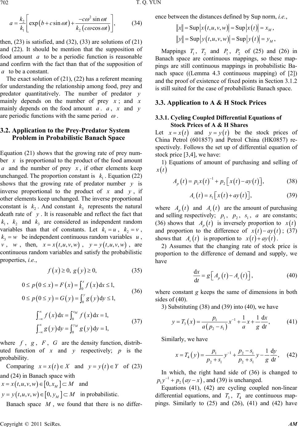

T. Q. YUN 702


2
2
12
sin
exp sin,
cos
kct
abct
kkc








t

(34)
then, (23) is satisfied, and (32), (33) are solutions of (21)
and (22). It should be mention that the supposition of
food amount to be a periodic function is reasonable
and confirm with the fact than that of the supposition of
to be a constant.
a
aThe exact solution of (21), (22) has a referent meaning
for understanding the relationship among food, prey and
predator quantitatively. The number of predator
mainly depends on the number of prey y
x
; and
x
mainly depends on the food amount . , a a
x
and
are periodic functions with the same period y

.
3.2. Application to the Prey-Predator System
Problem in Probabilistic Banach Space
Equation (21) shows that the growing rate of prey num-
ber
x
is proportional to the product of the food amount
and the number of prey a
x
, if other elements keep
unchanged. The proportion constant is 1. Equation (22)
shows that the growing rate of predator number is
inverse proportional to the product of
ky
x
and , if
other elements keep unchanged. The inverse proportional
constant is . And constant 3 represents the natural
death rate of . It is reasonable and reflect the fact that
1, 2 and 3
k are considered as independent random
variables than that of constants. Let 1, 2
y
kv
2
kyk
k kku

,
be independent continuous random variables ,
, , then,
3
k
vwwu

,,,
x
xtuvw,

,,

,
y
ytuvw, are
continuous random variables and satisfy the probabilistic
properties, i.e.,



0, 0,fx gy
1,
1,
1,
1,
(35)
 

0
0
00 d
00 d
x
y
pxFx fxx
pyGy gyy
 
 

 (36)
 
 
0
0
dd
dd
M
M
x
y
fx xfx x
gy ygy y







 (37)
where
f
,
g
,
F
, are the density function, distrib-
uted function of G
x
and respectively; is the
probability. y p
Comparing

x
xt X and

y
yt Y of (23)
and (24) in Banach space with
 

,,,0,M
x
xtuvwx M and
 

,,,0,M
y
ytuvwyM in probabilistic.
Banach space
M
, we found that there is no differ-
ence between the distanc e s d efined by Sup norm, i.e.,


 
Sup, , ,Sup,
Sup,, ,Sup,
M
M
x
xtuvwxt x
yytuvw yty




Mappings 1, 2 and 1, 2 of (25) and (26) in
Banach space are continuous mappings, so these map-
pings are still continuous mappings in probabilistic Ba-
nach space ((Lemma 4.3 continuous mapping) of [2])
and the proof of ex isten ce of fix ed po in ts in Section 3.1.2
is still suited for the case of probabilistic Banach space.
T TP P
3.3. Application to A & H Stock Prices
3.3.1. Cycli n g Co up l ed Di f ferential Equa tions of
Stock Prices of A & H Shares
Let


x
xt and


y
yt be the stock prices of
China Petrol (601857) and Petrol China (HK0857) re-
spectively. Follows the set up of differential equation of
stock price [3,4], we have:
1) Equations of amount of purchasing and selling of


x
t
 
1
12 , p
A
tpxtpxtayt



 
(38)




1, s
A
tsxtayt



 (39)
where


p
A
t and


s
A
tp
are the amount of purchasing
and selling respectively; 1, 2, 1 p
s
, are constants;
(36) shows that a


p
A
t is inversely proportion to


x
t
and proportion to the difference of



x
tayt; (37)
shows that


s
A
t is proportion to



x
tayt.
2) Assumes that the changing rate of stock price is
proportion to the difference of demand and supply, we
have
 
d
dps
x
g
At At
t

 

, (40)
where constant g keeps the same of dimensions in both
sides of (40).
3) Substituting (38) an d (39) into (40), we have
 
1 1
321
11d
,
d
p
x
yTxx x
apsagt

 
 (41)
Similarly, we have

1
121
421 21
1d ,
d
pps y
xTy yy
psps gt

 
 (42)
In which, the right hand side of (36) is changed to


1
12
pyp ayx


, and (39) is unchanged.
Equations (41), (42) are cycling coupled non-linear
differential equations, and 3, 4 are continuous map-
pings. Similarly to (25) and (26), (41) and (42) have
T T

T. Q. YUN703
fixed poi nt s and
34 43
**yTTy**
x
TTx.
If the coefficients in (41) and (42) are viewed as ran-
dom variables, then, and y
x
are the functions of
random variables, like the case in Section 3.2, and y
x
also have fixed points in probabilistic Banach space.
3.3.2. An Exact Solution of Speculating Type
Differential Equations of Stock Price for
A & H Stocks
Usually, (41), (42) may have no exact solution. However,
for a simplest case, for example, the second term in (38)
is much larger than the first term, i.e., the speculation on
the difference of stock prices in A & H stock market (and
suppose that there is no limit for money freely to pur-
chase a stock in A or H stock market) forms a major part
of the purchasing volume. In such case, , and (41),
(42) become 10p
11d
,
d
x
yx
ag
t (43)
21
21
1d ,
d
y
gt

ps
xy
ps


 (44)
Equations (43), (44) are cycling coupled differential
equations of stock prices in A and H stock markets.
Substituting (44) in to (43), we have
2
2
dd 0,y
d d
yy
RS
t t (45)
where

Rgakg,


2
kgSa, 21
21
p
ks
ps



.
Equation (45) has exact solution, depended on the root
of characteristic function .
2
rR 0rS

2 2
p ,
1) when ,
240RS

11
exp ex
y
CrtCrt (46)
where , are arbitrary constants, and
1
C2 C

2
1
rRR 42,S

2
242rRRS ,
2) When ,
240RS

exp, 2,yCrtr R
0
(47)
3) When , the characteristic function has
complex roots and there is no real meaning for has
complex value and thus is out of discussion.
24RS y
Similarly, substituting (43) into (44), we have,
2
2
dd 0,
d
d
xxS
Rx
ta
t
(48)
4) When 240RSa

,

 
3344
expexp ,
x
CrtCrt (49)
where , are arbitrary constants, and
3
C4 C

2
342rRRSa


 



,

2
442rRRSa

 


,
5) When 240RSa

,


55
exp, 2,xCrtr R (50)
6) When 240RSa

,
x
has no real meaning and
is out of discussion.
4. Discussion on the Solution
We are interested in “what is ” and “how to find ”. a a




*axt yt* is the ratio of A-share price to H-share
price at the equilib rium time . If , then the
“hot money” (money can freely purchase or sell stocks in
A and H markets) rushes into H-stock market to purchase
the cheaper shares; if
*t
0y
0xay
xa

, then the hot money
rushes into A-stock market to purchase the cheaper
shares. And if 0xay

, then it is the equilibrium state,
in which no profits can be made by speculating the dif-
ference of sto ck prices in A-stock or H-stock m a rke t s.
a is an important value for decision making of op-
erators. But how to find = ? a
From (41), if dd0xt

, then,



**axt yt.
From (42), if dd 0yt

, then, 11
 
x
tkyt. If both
stock prices are in equilibrium state at the same time
1
*tt

, then ak

.
The determination of coefficients via market data may
be referr ed to [3], or we can directly use the share prices
both in temporary equilibrium states (the so-called
“Doji” or the Chinese stock market saying “cross star”)
of A and H stock markets at the same time to find .
For example, 2008-04-10, a “Doji” for China Petrol
(601857) (op ening price 17.11, closing price 17.35 RMB)
and a near “Doji” for Petrol China (HK0857) (opening
price 10.20, closing price 9.82 HKD). Then, =
a
a
x
y
= 17.35×0.88/9.82 = 1.554. (where 0.88 is the changing
rate for RMB to HKD)
The analysis of this example might be useful to deci-
sion making of operators and is referred [6] for details.
5. References
[1] A. T. Bharucha-Reid, “Fixed Point Theorems in Prob-
abilistic Analysis,” Bulletin of the American Mathemati-
cal Society, Vol. 83, No. 5, 1976, pp. 641-657.
doi:10.1090/S0002-9904-1976-14091-8

T. Q. YUN 704
[2] T. Q. Yun, “Fixed Point Theorem of Composition
G-Conaction Mapping and Its Applications,” Applied
Mathematics and Mechanics, Vol. 22, No. 10, 2001, pp.
1132-1139. doi:10.1023/A:1016337014775
[3] J. S. Yu, T. Q. Yun and Z. M. Guo, “Theory of Computa-
tional Securities,” In Chinese, Scientific Publication
House, Beijing, 2008.
[4] T. Q. Yun and G. L. Lei, “Simplest Differential Equation
of Stock Price, Its Solution and Relation to Assumption
of Black-Scholes Model,” Applied Mathematics and Me-
chanics, Vol. 24, No. 6, 2003, pp. 654-658.
doi:10.1007/BF02437866
[5] C. W. Gardiner, “Handbook of Stochastic Methods, for
Physics, Chemistry and the Natural Sciences,” Springer-
Verlag Press, Berlin, 1983.
[6] T. Q. Yun and T. Yun, “Simple Differential Equations of
A & H Stock Prices and Application to Analysis of Equi-
librium Stat e,” Technology and Investment, Vol. 1, No. 2,
2010, pp. 111-114. doi:10.4236/ti.2010.12013