 Applied Mathematics, 2011, 2, 685-693 doi:10.4236/am.2011.26090 Published Online June 2011 (http://www.SciRP.org/journal/am) Copyright © 2011 SciRes. AM Soliton Resonances of the Nonisospectral Modified Kadomtsev-Petviashvili Equation Jiaojiao Yan Zhejiang Institute of Communications, Hangzhou, China E-mail: yanjj@zjvtit.edu.com Received March 24, 20 1 1; revised April 2, 2011; accepted April 5, 2011 Abstract Many equations possess soliton resonances phenomenon, this paper studies the soliton resonances of the nonisospectral modified Kadomtsev-Petviashvili (mKP) equation by asymptotic analysis. Keywords: Soliton, Resonances, Hirota Bilinear Method, Nonisospectral mKP Equation 1. Introduction In the process of searching for explicit solutions, quite a few systematic methods have been developed, such as inverse scattering transformation [1], Darboux transfor- mations [2], Hirota’s bilinear method [3-5], and so on. Among them, the bilinear method first proposed by Hi- rota provides us with a comprehensive approach to con- struct exact solutions of nonlinear evolution equations (NEEs). Meanwhile, as the interacting of the solution, soliton resonance has been studied in many papers. Miles obtained resonantly interacting solitary waves of KP equation [6], these solutions are coherent structures that describe the diffraction of a soliton at a corner, and sug- gest that, under certain conditions, a KP soliton can’t turn at a convex corner without separating or otherwise losing its identity. Thus, these structures provide a solu- tion of the problem of “Mach reflection” in water waves, and this phenomenon is now known as soliton resonance. Asymptotic analysis is a very important tool in studying the behaviors of soliton solu tions, we call the asymptotic line soliton solutions as and as the incoming and outgoing line soliton solutions, respec- tively. The amplitudes, directions and even the number of incoming solitons are in general different from those of the outgoing ones, wh en resonance occurs two soliton solutions under certain condition resonate and create a new soliton solutio n. y y Multisoliton solutions exhibiting nontrivial spatial structures and interaction patterns were found in many well-known soliton equations. Hirota studied resonances of solitons in one-dimensional space theoretically taking the Sawada-Kotera equation with a nonvanishing bound- ary condition as an example by his bilinear method [7], in which he pointed out that two solitons at the resonant state fused after colliding with each other, or a soliton splited into two solitons. Other (1 + 1)-dimensional space equations like KdV-SK and Hirota-Satsuma equations [8] and Boussinesq equation [9]. However more emphases are placed on (2 + 1)-dimen- sional ones, the most relevant with ours like the follow- ing: Wadati clarified the fundamental properties of the soliton in KP equation [1 0], Medina then went further in this equation [11], Pashaev created four virtual soliton resonance solution for KP-II [12], Biondini made use of tau-function in Wronskian to study it [13], after that Iso- jima studied the parameter regions for resonance and also study the “spider web”-like solution for cKP system [14,15], the approach of the Reference [16] for MKP-II equation allows audiences to interpret the resonance soliton as a composite object of two dissipative solitons in (1 + 1) dimensions, Hao investigated the resonance of two line solitons of the nonisospectral KP equation [17] which classified the resonance condition clearly. Reso- nance can also occur in (3 + 1)-dimensional system [18] and even multi-dimensional space [19,20]. In recent years, much attention has been paid to the study of nonisospectral systems [21], as nonisospectral evolution equations are of physical and mathematical importance, which can b e used to describe solitary waves in a certain type of non-uniform media with a relaxation effect. The aim of this paper is to clarify the fundamental properties of the soliton resonances in the (2 + 1)-dimen- sional nonisospectral mKP equation 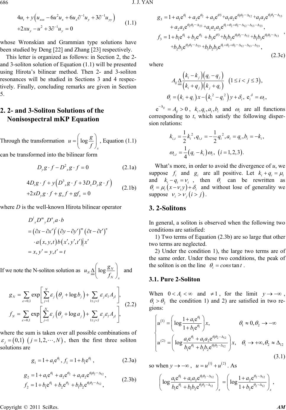 J. J. YAN 686 y 211 21 4663 230 txxx xxyy yy uyuuuu uu xu uu (1.1) whose Wronskian and Grammian type solutions have been studied by Deng [22 ] and Zhang [23] respectiv ely. This letter is organized as follows: in Section 2, the 2- and 3-soliton so lution of Equation (1 .1) will be presented using Hirota’s bilinear method. Then 2- and 3-soliton resonances will be studied in Sections 3 and 4 respec- tively. Finally, concluding remarks are given in Section 5. 2. 2- and 3-Soliton Solutions of the Nonisospectral mKP Equation Through the transformation log u , Equation (1.1) can be transformed into the bilinear form 20 yx Dg fDg f (2.1a) 3 43 20 txxy yxx Dg fyD g fDDgf xDgf gf gf (2.1b) where D is the well-known Hirota bilinear operator ,,,, ,, lmn xyt lm DD Dab n xyy tt axytbxyt x xyytt If we note the N-soliton sol ution as log N NN g uf ljl ljl A A N 1 , 12 , and 0,111 0,111 exp log, exp log, N Njjjj jjl N Njjjj jjl gb fa (2.2) where the sum is taken over all possible combinations of , then the first three soliton solutions are 0,1 1,2,, jj 1 1111 1e, 1egafb (2.3a) 12 12 12 1212 21212 21212 1e ee 1e ee, gaaaa fbbbb - - (2.3b) 13 13 12 1212 23231 2 3121323 13 13 12 1212 23231 2 31213 3 31231213 23 123 3 312312 13 23 123 1e eeee ee, 1e eeee ee gaaaaa aa aa aaa fbbbbbbb bb bbb - - -- - - -- ++ + ++ ++ 23 , , (2.3c) where 13 ijij ij ijji kkqq Ai kqkq ,j 22 , e, iiiiiii kqxk qy i ij e0A ij , and i ,,, iiii kqab are all functions corresponding to t, which satisfy the following disper- sion relations: 22 ,, , 11 ,,, 22 1, 1,2,3. 4 itiitiiiii itii i kkq qaqbk qk i , What’s more, in order to avoid the divergence of u, we suppose i and i are all positive. Let iii kq and ii kq i , then i can be rewritten as ii i xyi and without lose of generality we suppose j ij i. 3. 2-Solitons In general, a soliton is observed when the following two conditions are satisfied: 1) Two terms of Equation (2.3b) are so large that other two terms are neglected. 2) Under the condition 1), the large two terms are of the same order. Under these two conditions, the peak of the soliton is on the line tan icons t . 3.1. Pure 2-Soliton When 0i A and 1 , for the limit , 12 y the condition 1) and 2) are satisfied in two re- gions: 1 1 11212 11212 1112 1 (2) 11212 112 1e log, 0, 1e ee log, , ee a ux b aaa ux bbb 12 (3.1) so when, . As y 1 uu u 2 11212212 11212212 112 2 112 2 ee 1e loglog , ee 1e x aaa a bbb b Copyright © 2011 SciRes. AM 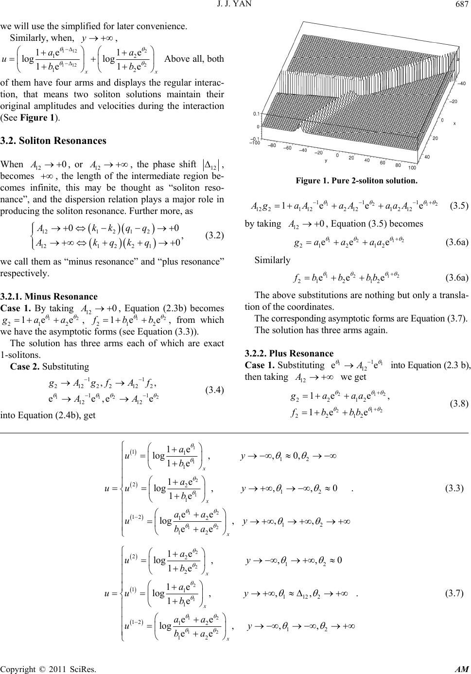 J. J. YAN Copyright © 2011 SciRes. AM 687 we will use the simplified for later convenience. Similarly, when, , y 112 2 112 2 1 12 1e 1e log log 1e 1e 2 x a ubb a Above all, both of them have four arms and displays the regular interac- tion, that means two soliton solutions maintain their original amplitudes and velocities during the interaction (See Figure 1). 3.2. Soliton Resonances When 12, or 12 , the phase shift 0A A 12 , becomes , the length of the intermediate region be- comes infinite, this may be thought as “soliton reso- nance”, and the dispersion relation plays a major role in producing the soliton resonance. Further more, as Figure 1. Pure 2-soliton solution. 12 11 1 1221 122121 212 1e eeAgaAaAaaA 12 (3.5) 121 2 12 121 22 1 0, 0 Akkqq Akqkq 0 (3.2) by taking , Equation (3.5 ) becomes 12 0A 12 1 21 212 ee egaaaa2 2 (3.6a) Similarly we call them as “minus resonance” and “plus resonance” respectively. 12 1 21 212 ee efb bbb 1 e (3.6a) The above substitutio ns are nothing but only a transla- tion of the coordinates. 3.2.1. Min u s Res o nance Case 1. By taking 12 , Equation (2.3b) becomes 212 0A 12 ea1ega , 1 212 1e efbb The corresponding asymptotic forms are Equati on (3.7). 2 , from which we have the asymptotic forms (see Equation (3.3)). The solution has three arms again. The solution has three arms each of which are exact 1-solitons. 3.2.2. Plus R esonance Case 1. Substituting 12 1 1 eA into Equation (2.3 b), then taking we get 12 A Case 2. Substituting 112 11 21222122 1 12 12 ,, ee,e 2 1 e Agf Af AA (3.4) 21 21 2212 2212 1e e 1e e gaaa fbbb 2 2 , (3.8) into Equatio n (2.4b), get 1 1 2 1 12 12 1112 1 2212 1 12 12 12 12 1e log, ,0, 1e 1e log, ,,0. 1e ee log, ,, ee x x x a uy b a uu y b aa uy ba (3.3) 2 2 2 1 12 12 2212 2 111122 1 12 12 12 12 1e log, ,,0 1e 1e log, ,,. 1e ee log, ,, ee x x x a uy b a uu y b aa uy ba (3.7) 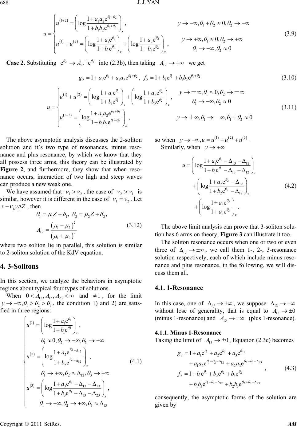 J. J. YAN 688 12 12 12 12 12 12 12 2 12 12 12 12 12 12 1e log, ,0, 1e ,0, 1e 1e loglog, ,0 1e 1e x xx aa uy bb uy aa uu bb 2 e (3.9) Case 2. Substituting 2 1 12 eA into (2.3b), then taking we get 12 A 1121 21122112 1ee, 1eegaaa fbbb 12 (3.10) 12 12 12 12 12 12 12 12 12 12 12 112 12 ,0, 1e 1e loglo g, ,0 1e 1e 1e log, ,,0 1e xx x y aa uu bb uaa uy bb -- +-+ (3.11) The above asymptotic analysis discusses the 2-soliton solution and it’s two type of resonances, minus reso- nance and plus resonance, by which we know that they all possess three arms, this theory can be illustrated by Figure 2, and furthermore, they show that when reso- nance occurs, interaction of two high and steep waves can produce a new weak one. We have assumed that 12 , the case of 12 12 is similar, however it is different in the case of . Let 1 yZ , then 111222 2 12 12 2 12 , ,ZZ A (3.12) where two soliton lie in parallel, this solution is similar to 2-soliton solution of the KdV equation. 4. 3-Solitons In this section, we analyze the behaviors in asymptotic regions about typical four types of solutions. When and , for the limit 123 12 1323 0,,AAA1 , y , the condition 1) and 2) are satis- fied in three regions: 1 212 212 3 3 111 1 12 3 22 2 12123 331323 31323 1e log, 1e 0,, 1e log, 1e ,, 1e log, 1e x x x a ub a ub a ub 1231 ,, 3 3 u (4.1) so when . 12 ,yuuu y Similarly, when 1 1 2 2 3 3 11312 11312 212 212 3 3 1e log 1e 1e log1e 1e log. 1e x x a ub a b a a (4.2) The above limit analysis can prove that 3-soliton so lu- tion has 6 arms on theory, Figure 3 can illustrate it too. The soliton resonance occurs when one or two or even three of ij , we call them 1-, 2-, 3-resonance solution respectively, each of which include minus reso- nance and plus resonance, in the following, we will dis- cuss them all. 4.1. 1-Resonance In this case, one of ij , we suppose 13 0 A without lose of generality, that is equal to 13 (minus 1-resonance) and (plus 1-resonance). 13 A 4.1.1. Minus 1-Resonance Taking the limit of , Equation (2.3c) becomes 13 0A 31 12 23 23 1212 122 23 23 1212 3123 12 23 2123 13 23 1e ee ee 1e ee ee gaaa aa aa fbbb bb bb , (4.3) consequently, the asymptotic forms of the solution are iven by g Copyright © 2011 SciRes. AM 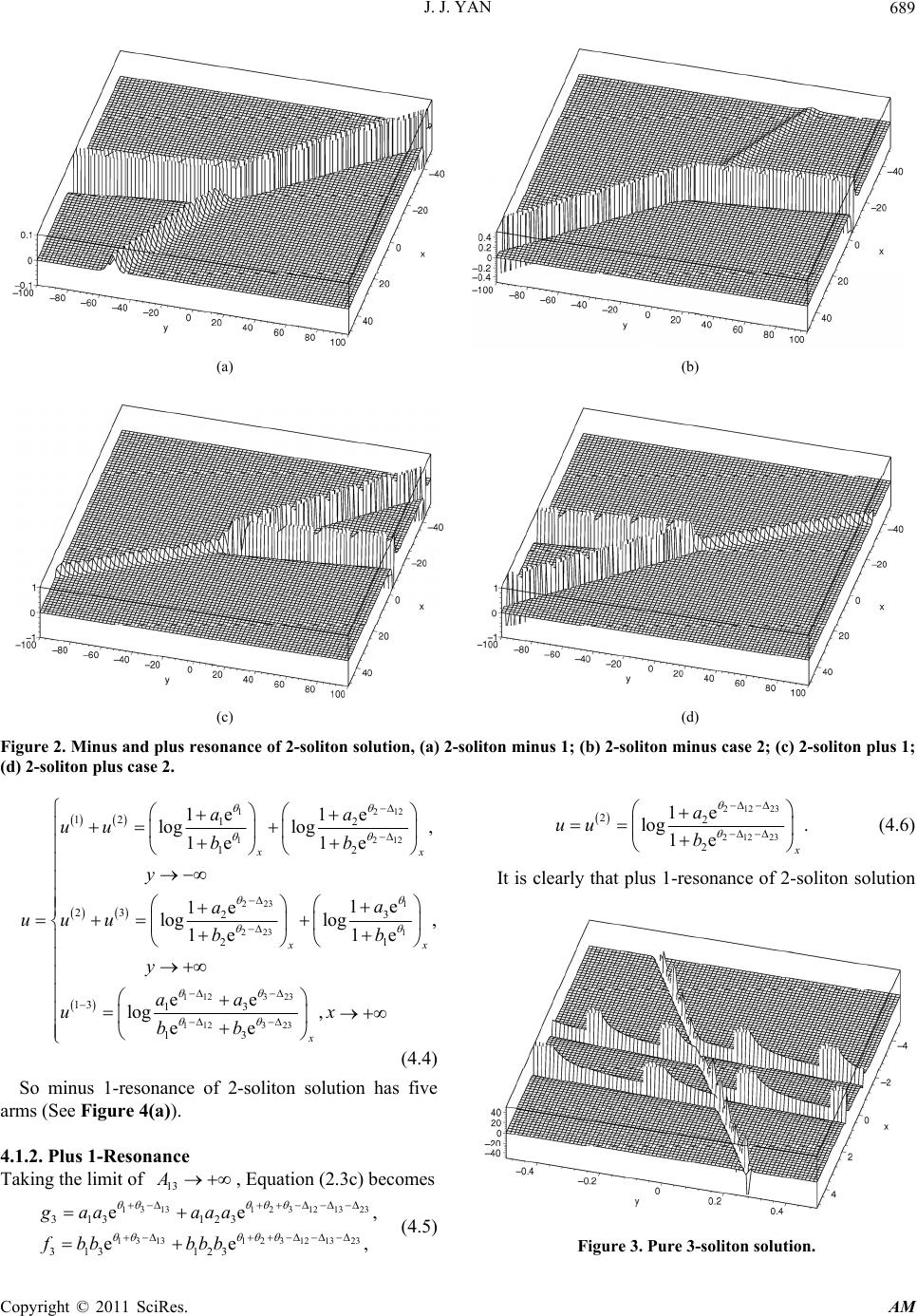 J. J. YAN Copyright © 2011 SciRes. AM 689 (a) (b) (c) (d) Figure 2. Minus and plus resonance of 2-soliton solution, (a) 2-soliton minus 1; (b) 2-soliton minus case 2; (c) 2-soliton plus 1; (d) 2-soliton plus case 2. 12 12 1223 223 1 32 112 12 12 12 23 3 2 1 2 13 13 1e 1e log log, 1e 1e 1e 1e loglog , 1e 1e ee log 12 12 x x aa uu bb y a a uu ub b y aa u 3 323 112 13 , ee x x bb (4.4) So minus 1-resonance of 2-soliton solution has five arms (See Figure 4(a)). 4.1.2. Plus 1-Resonance Taking the limit of , Equation (2 . 3c) becomes 13 A 13 13123 12 1323 131312312 13 23 313 123 313 123 ee ee gaa aaa fbbbbb 21223 212 23 22 2 1e log . 1e a uu b (4.6) It is clearly that plus 1-resonance of 2-soliton solution , , (4.5) Figure 3. Pure 3-soliton solution.  J. J. YAN 690 3 only has one arm, and the figure is similar to that of 1-solition solution. 4.2. 2-Resonance In this case, two of ij , w e suppose 12, 23 without lose of generality, which are equal to (minus 2-resonance) and (plus 2-resonance). 12 12 , 23 0, 0 23 4.2.1. Plus 2-Resonance Case 1. Substituting 3 22 12 23 ee, eeAA 12 into Equation (2.3c), and taking the limit of and 13 , we get 12313 112 12313 112 3112 123 3112123 1e ee 1e ee ga aaaaa fbbbbbb (4.7) Then 313 313 21 21 12313 12313 321 3 3 21 21 123 123 123 1e log 1e 1e 1e log(log),, 1e 1e 1e log, . 1e x x x x a uuu b aa uy bb aaa uy bbb 2 (4.8) Case 2. Substituting 11 2 12 23 ee,eeAA 12 into Equation (2.3c), and taking the limit of and 23 , we get 323 123 323123 3323 123 3323 123 1e ee 1e ee gaaaaaa fbbb bbb 13 13 , (4.9) Then 32 3 13 1 13 1 12313 12313 321 32 2 3 1 1 123 123 123 1e 1e loglog 1e 1e 1e log, 1e 1e log , 1e 2 x x x aa uuu b b a u b aaa uy bbb y 2 (4.10) Case 3. Substituting 2 12 23eeAA 12 into Equation (2.3c), and taking the limit of and 23 , we get 313 1 12313 313 1 12 313 31313 123 313 13 123 1e ee e 1e ee e gaaaa aaa fbbbb bbb Then 3 3 12 13 12 13 1 1 2313 2313 312 3 3 12 12 1231 1 23 23 1e log 1e 1e log, 1e 1e log 1e 1e log, 1e x x x x a uu b aa y bb ua uu b aa y bb (4.12) 4.2.2. Minus 2-Resonance In the limit of Equation (2.3c) can be rewritten as 12 23 0, 0,AA 313 12 313 12 312313 312313 1e eee 1e eee gaaaaa fbbbbb 13 13 , (4.13) Then 3 2 3 2 113 113 313 313 1 1 23 123 23 1 1 31 3 3 1 1 ee log ee 1e log, 1e 1e log 1 1e log, 1e x x x x aa uu bb ay b ua uu b ay b , (4.14) The case of condition 12 and 13 , 13 23 , are similar. By the asymptotic analysis above, we know that two types of 2-resonance 3-so liton solution possess four arms (See Figures 4(b)-(d)), the 2-soliton solution has also four arms, but differently, the behaviors of the former in the intermediate region are not stationary. 4.3. 3-Resonance For the plus 3-resonance, substituting 11 12eeA, 3 22 23 13 ee,eeAA 3 12 into Equation (2.3c), and taking the limit of , we get 13 23 ,,AA A 123 123 3123 3123 1e 1e gaaa fbbb (4.15) 13 13 (4.11) this case is like 1-soliton solution, which only has one arm. For the minus 3-resonance, by taking the limit Copyright © 2011 SciRes. AM  J. J. YAN Copyright © 2011 SciRes. AM 691 (a) (b) (c) (d) (e) (f) Figure 4. Minus and plus resonance of 3-soliton solution, (a) 3-soliton minus 1-resonance; (b) 3-soliton plus 2-resonance case 1; (c) 3-soliton plus 2-resonance case 2; (d) 3-soliton plus 2-resonance case 3; (e) 3-soliton minus 2-resonance; (f) 3-soliton inus 3-resonance. m 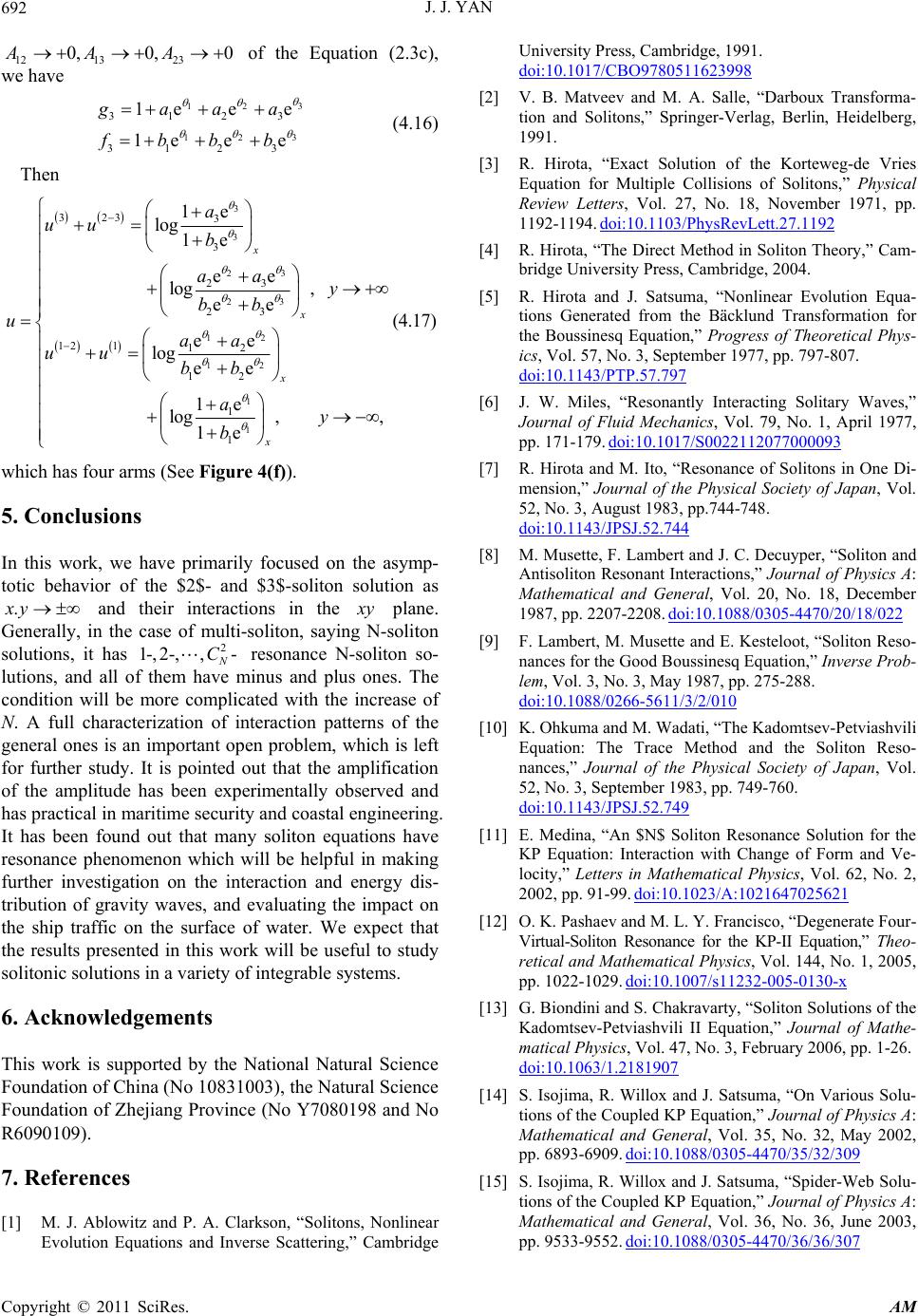 J. J. YAN Copyright © 2011 SciRes. AM 692 12 1323 0, 0,0AAA of the Equation (2.3c), we have 3 12 3 12 3123 3123 1e ee 1e ee gaaa fbbb (4.16) Then 3 3 3 2 3 2 12 12 1 1 3233 3 23 23 12 112 12 1 1 1e log1e ee log, ee ee log ee 1e log,, 1e x x x x a uu b aa y bb uaa uu bb ay b (4.17) which has f ou r arms (See Figure 4(f)). 5. Conclusions In this work, we have primarily focused on the asymp- totic behavior of the $2$- and $3$-soliton solution as and their interactions in the .xy y plane. Generally, in the case of multi-soliton, saying N-soliton solutions, it has 2 1-, 2-,,- C resonance N-soliton so- lutions, and all of them have minus and plus ones. The condition will be more complicated with the increase of N. A full characterization of interaction patterns of the general ones is an important open problem, which is left for further study. It is pointed out that the amplification of the amplitude has been experimentally observed and has practical in maritime security and coastal engineering. It has been found out that many soliton equations have resonance phenomenon which will be helpful in making further investigation on the interaction and energy dis- tribution of gravity waves, and evaluating the impact on the ship traffic on the surface of water. We expect that the results presented in this work will be useful to study solitonic solutions in a variety of integrable systems. 6. Acknowledgements This work is supported by the National Natural Science Foundation of China (No 10831003), the Natural Science Foundation of Zhejiang Province (No Y7080198 and No R6090109). 7. References [1] M. J. Ablowitz and P. A. Clarkson, “Solitons, Nonlinear Evolution Equations and Inverse Scattering,” Cambridge University Press, Cambridge, 1991. doi:10.1017/CBO9780511623998 [2] V. B. Matveev and M. A. Salle, “Darboux Transforma- tion and Solitons,” Springer-Verlag, Berlin, Heidelberg, 1991. [3] R. Hirota, “Exact Solution of the Korteweg-de Vries Equation for Multiple Collisions of Solitons,” Physical Review Letters, Vol. 27, No. 18, November 1971, pp. 1192-1194. doi:10.1103/PhysRevLett.27.1192 [4] R. Hirota, “The Direct Method in Soliton Theory,” Cam- bridge University Press, Cambridge, 2004. [5] R. Hirota and J. Satsuma, “Nonlinear Evolution Equa- tions Generated from the Bäcklund Transformation for the Boussinesq Equation,” Progress of Theoretical Phys- ics, Vol. 57, No. 3, September 1977, pp. 797-807. doi:10.1143/PTP.57.797 [6] J. W. Miles, “Resonantly Interacting Solitary Waves,” Journal of Fluid Mechanics, Vol. 79, No. 1, April 1977, pp. 171-179. doi:10.1017/S0022112077000093 [7] R. Hirota and M. Ito, “Resonance of Solitons in One Di- mension,” Journal of the Physical Society of Japan, Vol. 52, No. 3, August 1983, pp.744-748. doi:10.1143/JPSJ.52.744 [8] M. Musette, F. Lambert and J. C. Decuyper, “Soliton and Antisoliton Resonant Interactions,” Journal of Physics A: Mathematical and General, Vol. 20, No. 18, December 1987, pp. 2207-2208. doi:10.1088/0305-4470/20/18/022 [9] F. Lambert, M. Musette and E. Kesteloot, “Soliton Reso- nances for the Good Boussinesq Equation,” Inverse Prob- lem, Vol. 3, No. 3, May 1987, pp. 275-288. doi:10.1088/0266-5611/3/2/010 [10] K. Ohkuma and M. Wadati, “The Kadomtsev-Petviashvili Equation: The Trace Method and the Soliton Reso- nances,” Journal of the Physical Society of Japan, Vol. 52, No. 3, September 1983, pp. 749-760. doi:10.1143/JPSJ.52.749 [11] E. Medina, “An $N$ Soliton Resonance Solution for the KP Equation: Interaction with Change of Form and Ve- locity,” Letters in Mathematical Physics, Vol. 62, No. 2, 2002, pp. 91-99. doi:10.1023/A:1021647025621 [12] O. K. Pashaev and M. L. Y. Francisco, “Degenerate Four- Virtual-Soliton Resonance for the KP-II Equation,” Theo- retical and Mathematical Physics, Vol. 144, No. 1, 2005, pp. 1022-1029. doi:10.1007/s11232-005-0130-x [13] G. Biondini and S. Chakravarty, “Soliton Solutions of the Kadomtsev-Petviashvili II Equation,” Journal of Mathe- matical Physics, Vol. 47, No. 3, February 2006, pp. 1-26. doi:10.1063/1.2181907 [14] S. Isojima, R. Willox and J. Satsuma, “On Various Solu- tions of the Coupled KP Equation,” Journal of Physics A: Mathematical and General, Vol. 35, No. 32, May 2002, pp. 6893-6909. doi:10.1088/0305-4470/35/32/309 [15] S. Isojima, R. Willox and J. Satsuma, “Spider-Web Solu- tions of the Coupled KP Equation,” Journal of Physics A: Mathematical and General, Vol. 36, No. 36, June 2003, pp. 9533-9552. doi:10.1088/0305-4470/36/36/307  J. J. YAN693 [16] J. H. Lee, R. Willox and O. K. Pashaev, “Soliton Reso- nances for the MKP-II,” Theoretical and Mathematical Physics, Vol. 144, No. 1, July 2005, pp. 995-1003. doi:10.1007/s11232-005-0127-5 [17] H. H. Hao and D. J. Zhang, “Resonances of Line Solitons in a Non-Isospectral Kadomtsev-Petviashvili Equation,” Journal of the Physical Society of Japan, Vol. 77, April 2008, Paper ID: 045001. doi:10.1143/JPSJ.77.045001 [18] L. M. Alonso, E. L. Medina and R. Hernandez, “Multi- dimensional Localized Coherent Structures in the Bilin- ear Formalism of Integrable Systems,” Inverse Problem, Vol. 7, No. 3, June 1991, p. L25. doi:10.1088/0266-5611/7/3/001 [19] F. Kaka and N. Yajima, “Interaction of Ion-Acoustic Solitons in Two-Dimensional Space,” Physical Society of Japan, Vol. 49, November 1980, pp. 2063-2071. doi:10.1143/JPSJ.49.2063 [20] F. Kaka and N. Yajima, “Interaction of Ion-Acoustic Solitons in Multi-Dimensional Space II,” Physical Soci- ety of Japan, Vol. 51, January 1982, pp. 311-322. doi:10.1143/JPSJ.51.311 [21] Y. Zhang, S. F. Deng, D. J. Zhang and D. Y. Chen, “The N-Soliton Solutions for the Non-Isospectral Mkdv Equa- tion,” Vol. 339, No. 3-4, August 2004, pp. 228-236. [22] S. F. Deng, “The Multisoliton Solutions for the Noniso- spectral mKP Equation,” Physics Letters A, Vol. 372, No. 4, January 2008, pp. 460-464. doi:10.1016/j.physleta.2007.07.060 [23] Y. Zhang and Y. N. Lv, “On the Nonisospectral Modified Kadomtsev-Peviashvili Equation,” Journal of Mathe- matical Analysis and Applications, Vol. 342, No. 1, June 2008, pp. 534-541. doi:10.1016/j.jmaa.2007.12.032 Copyright © 2011 SciRes. AM
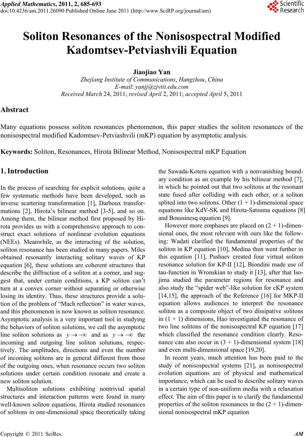
|