 Journal of Applied Mathematics and Physics, 2014, 2, 869-874 Published Online August 2014 in SciRes. http://www.scirp.org/journal/jamp http://dx.doi.org/10.4236/jamp.2014.29098 How to cite this paper: El-Shal, A.O., Mansour, N.A., Taha, M.M., Qandil, O.S.A. (2014) Hartree-Fock Calculations of 16O and 40Ca Nuclei Using Fish-Bone Potential. Journal of Applied Mathematics and Physics, 2, 869-874. http://dx.doi.org/10.4236/jamp.2014.29098 Hartree-Fock Calculations of 16O and 40Ca Nuclei Using Fish-Bone Potential Azza O. El-Shal1, N. A. Mansour2, M. M. Taha1, Omnia S. A. Qandil1 1Mathematics and Theoretical Physics Department, Nuclear Research Center, Atomic Energy Authority, Cairo, Egypt 2Physics Department, Faculty of Science, Zagazig University, Zagazig, Egypt Email: azshal@hotmail.com Received 24 Ju ly 2014 Abstract Hartre e-Fock calculations are carried out to describe some properties of 16O and 40Ca nuclei using the two forms of fish-bone potential (I and II). A computer simulation search program has been introduced to solve this problem. The Hilbert space was restricted to three dimensional variational space spanned by single spherical harmonic oscillator orbits. Binding energies, root mean square radii and form factors are found to have a good fit with experimental data. Keywords Nuclear Structure, Hart ree -Fock Theory, Fish -Bone P oten ti al 1. Introduction The Hartree-Fock (HF) theory [1]-[3] and more elaborate self-consistent theories [4] [5] have been widely and successfully applied to investigate various properties of nuclear structure. Also the problem of cluster structure in nuclei has been a subject of interest since the early days of nuclear physics till now [6]. The idea is largely supported by the fact that alpha particles have exceptional stability and that they are the heaviest particles emit- ted in natural radioactivity. Various models have been proposed to account for possible nuclear clustering and to study its effects [7]. Later, a simple version of the model, in which the alphas are assumed to have no internal struc ture , is considered. The concept of clustering is very widely used in physics. The concept of alpha- cluster- ing has found many applications to nuclear reactions and nuclear structures [8] [9]. Many such clusters are possible in principle, but the formation probability depends on the stability of the cluster, and of all possible clusters the alpha particle is the most stable due to its high symmetry and binding energy. Thus a discussion of clustering in nuclei is mainly confined to alpha-particle clustering. For the α-nuclei 8Be, 12C, 16O, 20Ne, 24Mg, 28Si, 32S, the geometrical equilibrium configuration of the α-particles are generally assumed to belong to the symmetry point groups D∞h, D3h, Td, D3h, Oh (or alternatively D4h), D5h, D6h, respectively. The fishbone potential [10] of composite particles simulates the Pauli effect by nonlocal terms. The α-α fish- bone potential be determined by simultaneously fitting to two-α resonance energies, experimental phase shifts,  A. O. El-Shal et al. and three-α binding energies. It was found that, essentially, a simple Gaussian can provide a good description of two-α and three-α experimental data without invoking three-body potentials. Many authors adopted the fishbone model because, in their opinion, this is the most elaborated phenomenological cluster-model-motivated potential. The variant of the fishbone potential has been designed to minimize and to neglect the three-body potential. Therefore, they can try to determine the interaction by a simultaneous fit to two- and three-body data [11]. 2. The Theory We consider a system of N identical bosons described by a Hamiltonian of the usual form 11 ˆ ˆ()(, ) NN i ij HTVtivi j = ≠= =+=+ ∑∑ (1) where t(i) is the kinetic energy operator ith particle and v(i, j) the two-body interaction. In Hartree-Fock method, one takes for the best choice of the normalized wave function ψ the one that it minimizes the expectation value of the Hamiltonian H (2) In most Hatree-Fock calculations for light nuclei one has taken the subspace spanned by the lowest harmonic oscillator shell l j>. We assume that all the particles occupy the same orbital λ belonging to the average field. Hence the intrinsic state of the whole system would be described by the symmetric wave function (1,2,.....,)(1)(2) (3).........()NN ψλλ λλ = (3) In this subspace, the HF orbitals l λ > are then determined by their expansion coefficients . (4) And the HF-Hamiltonian h ( λ 1, λ 2, ….. λ N) is replaced by the matrix kl s kl i hji tjmikvjlm λλ λ ∗ =+ ∑∑∑ (5) whe re (6) The HF Equations are then replaced by the matrix Equation (7) One proceeds by iteration until self-consistency is achieved. 3. Fish-Bone Potential A fishbone potential of the α-α system was determined by Schmid E. W. [12] [13] [14]. The harmonic oscillator width parameter was fixed to a = 0.55 fm−2 and. The local potential was taken in the form 2 2 042 ( )exp()() 3 lea V rvrerfr r β = −+ (8) where v0 = −108.41998 MeV and β = 0.18898 fm-2 and called Fish-Bone I ( FB -1) While this potential provides a reasonably good fit to l = 0 and l = 2 and l = 4 partial wave phase shifts, it seriously over binds the three-α sys- tem as shown in (Table 1). The experimental binding energy of the three-α (12C) system is E3α = −7.275 MeV. One may conclude that there is a need for three-body potential. This was the choice Oryu and Kamada [15]. They added a phenomenological three-body potential to the fish-bone potential of Kircher and Schmid [12] [13] [14] and found that a huge three-body potential is needed to reproduce the experimental data. But, Faddeev cal- culations [11] reveal that the = 4 partial wave is very important to the three-α binding and, for this partial wave, the fit to experimental data is not so stellar. So Papp Z. and Moszkowski S. [11] concluded, that it may be  A. O. El-Shal et al. Table 1. L = 0 three-binding energy as a function of subsystem angular momentum lmax in case if fish-bone potential of Kircher and Schmid (FB-1) [12] [13] [14] and the results of Papp Z. and Moszko wski S. (FB-2) [11]. lmax FB-1 FB-2 4 −15.47 −7.112 6 −15.63 −7.273 possible to improve the agreement in the = 4 partial wave and achieve a better description for the three-α binding energy in the point view of the these authors. Thus as a local potential, two Gaussians plus screened Coulomb potential are added to form Fish-Bone II (FB-2): 2 22 1 122 42 ( )exp()exp()() 3 l ea V rvrvrerfr r ββ = −+−+ (9) where v1, β1, v2, β2 and a are fitting parameters. In the fitting procedure Papp Z. and Moszkowski S. incorporated the famous 8Be, l = 0 resonance state at = (0.0916 − 0.000003i) MeV, the 12C three-α ground state energy = −7.275 MeV, and the l = 0, l = 2 and l = 4 low energy phase shifts. With parameters v1 = −120.30683493 MeV, β1 = 0.20206127 fm−2, v2 = 49.06187648 MeV, β2 = 0.76601097 fm−2 and a = 0.64874009 fm−2, they achieved a perfect fit. For the l = 0 two-body resonance state they get E2b = 0.09161 - 0.00000303i MeV, and for the three-body ground state E3b = −7.27502 MeV. Notice that unlike with the Ali-Bodmer potential, they achieved this agree- ment by using the same potential in all partial waves. Having this new α-α fish-bone potential from the fitting procedure, they also calculated the first excited state of the three-system. This state is a resonant state, and we got = (0.54 - 0.0005i) MeV, which is again very close to the experimental value. 4. Solutions in a Three-Dimensional Space We consider solutions in a three dimensional variational space spanned by the orthonormal states l 1>, l 2 > and l 3>. In this case, we have twenty-one different symmetrized two-body matrix elements. A HF-orbital λ will have the general form (10) whe re , jjjj jj j mm mm λλ λλ λλ λ δδ ′ ∗∗ ′ ′′ = = ∑∑ (11) And assume that the coefficient mj’s are real. To investigate the HF-solutions, we have to specify the alpha-alpha potential. The specific combinations cho- sen as the basic states depend on the symmetry of the intrinsic structure that is expected from the molecular al- pha-particle model. Now we chose basic states which are invariant with respect to the transformation of the symmetry group Td. Therefore, we chose our three basic states as (12) (13) {} 2 1 300(0404 ) 2g gg η η =+ +− + (14) where η is a parameter determined from the Td symmetry. Here the oscillator shell model wave functions are given by  A. O. El-Shal et al. (15) 1/2 31/2 2222 00 00 ()2(1)/(3/ 2)(/)(/)exp(/ 2) nn RrnnrL rr ββ ββ + =Γ+ Γ++×− (16) β 0 = (h/m αω )1/2 is the oscillator parameter. 5. Matrix Elements of the Kinetic and Potential Energy Considering HF-solutions with mixed parity (where it is important in nuclear calculations), therefore, we have only twelve non-vanishing two-body matrix elements for the potential energy vijkl and three matrix elements of kinetic energy namely t11, t22 and t33. Therefore the non-vanishing HF-Hamiltonian will be 222 11111111 1121221313 3 1 /2(1)h tNvmvmvm =+− ++ (17) ( ) ( ) 122111221221121223132223 1 /2(1)h hNvvmm vvmm == −+++ (18) ( ) 22 1331123221333 3113313311 3 1 /2(1)hhNv mv mvvmm == −+++ (19) ( ) 23322231 122233233223 1 /2(1)hhNv mmvvmm ==−++ (20) 2 222 2222212112222232332123 13 1 /2(1)2h tNvmvmvmvmm =+−++ + (21) 2 222 3333313113232333333133 13 1 /2(1)2h tNvmvmvmvmm =+−++ + (22) 6. Nuclear Density and Form Factor The parity projected part of the nuclear density distribution, normalized to unity, which corresponds to a HF- solution as defined by Equations (5)-(7), is found to be 32/326622 2222 00102 300 ()(1/)(8 /105)(/)(2/9)exp(/)rmrm mrr ρ βπβββ =+ +− (23) The form factor corresponding to the spherical part of the density distribution (24) is 2222 44226622 0023 023023 882 22 03 0 ()[1(34) / 6(2) /120(4)/840 /15120]exp(/ 4) Fqqmmqmmqmm qm q ββ β ββ =−+++−+ +− (24) where q is the momentum transfer. The expression of F0(q) has to be multiplied by a form factor F(q) = exp(−q2 β 2 α /4), which account for the α -particle distribution. 7. Discussion By using the two types of the Fish-Bone potentials I and II and with the oscillator parameter β0 for 16O and 40Ca in addition to the parameter of the alpha particle βα, we have got the nuclear structure properties of the 16O and 40Ca nuclei such as binding energies, root mean square radii and form factors, and comparing the results with the experimental elastic scattering charge form factor [16] and other theoretical ones such as HF (Hrtree-Fock using Skyrme-type wave function) [17], HO + SRC (Harmonic Oscillator + Short range correlation ) and HO (Har- monic Oscillator potential) [17]. Using the Fish-Bone potential I (FB-1) according to its Equation (8), the parameters used in our calculations of fishbone potential I of 16O and 40Ca are given in Table 2. The results of the binding energies and root mean square radii of 16O and 40Ca nuclei are given in Table 3. Using the Fish-Bone potential II (FB-1) as in Equation (9), the parameters used in our calculations of fishbone potential II of 16O and 40Ca are given in Table 4. The results of the binding energies and root mean square radii of 16O and 40Ca nuclei using Fish-Bone Potential II are given in Table 5.The charge form factor of 16O and 40Ca nuclei using Fi s h-Bone Potential II are given in Figure 1 and Figure 2. In case of Fish–Bone potential I (FB-1), the binding energy of 16O and 40Ca nuclei and the root mean square radii are in good agreement with the experimental results as shown in Table 3. But we have not got form factors for both nuclei. The reason of that is obvious because the potential FB-1 have no repulsive part. Applying the repulsive part v2 in the Fish-Bone potential II, we have got form factors for 16O and 40Ca nuclei as shown in 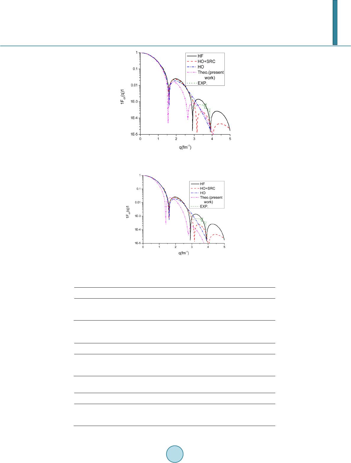 A. O. El-Shal et al. Figure 1. Charge form factors of 16O nuclei using the fish-bone potential II. Figure 2. Charge form factors of 40Ca nuclei using the fish-bone potential II. Table 2. The parameters used in our calculations of fishbone potential I of 16O and 40Ca. Nucleus V0 (MeV) β1 (fm−2) a (fm−2) 16O −11 0.1889 0.55 40Ca −13 0.1889 0.55 Table 3. The calculated binding energies and root mean square radii of 16O and 40Ca using the fish-bone potential I. Nucleus Theor. B. E. (MeV) Exp . B. E. (MeV ) Theor. rms (fm) Exp. Rms (fm) 16O −14.55 −14.40 2.55 2.7 40Ca −63.74 −62.047 3.24 3.49 Table 4. The parameters used in our calculations of fish-bone potential II of 16O and 40Ca. Nucleus V1 (MeV) V2 (M eV ) β1 (fm−2) β2 (fm−2) a (fm−2) 16O −51 135 0.2 021 0.7 660 0.6487 40Ca −60 180 0.2021 0 .7660 0.6487  A. O. El-Shal et al. Table 5. The calculated binding energies and root mean square radii of 16O and 40Ca using the fish-bone potential II. Nucleus Theor. B.E. (MeV ) Exp.B.E. (MeV) Theor. rms (fm) Exp. Rms (fm) 16O −13.9207 −14.40 2.7991 2.71 40Ca −62.7059 −62.047 3.24 3.49 Figure 1 and Figur e 2, which are in acceptable agreement with the experimental points in addition to other theoretical ones. Table 4 shows the parameters of the (FB-2) potential which gives us the binding energies and the root mean square radii of 16O and 40Ca, and we found that these values are in good agreement with the expe- rimental data (Table 5). References [1] Ri pka, G., Baranger, M. and Vogt, E. (1968) Advances in Nuclear Physics, 1. Phenum. [2] Guleria, N., Dhiman, S.K. and Shyam, R. (2012) A study of Λ Hypernuclei within the Skyrme-Hartree-Fock Model. Nuclear Physics A, 886, 71-91. [3] Sekiza wa, K. and Yabana, K. (2013) Ar-xiv: 1303.0552 [nucl-th] [4] Ri pka, G. and Porneuf, M. (1976) Proceedings of the International Conference on Nuclear Self-Consistent Fields, North Holland. [5] Gnezdilov, N.V., Borzov, I.N. , Saperstein, E.E. and Tolokonnikov, S.V. (2014 ) Ar x i v :1401.1319v4 [nucl-th] [6] Mo szko wski , S.A. (1957) Encyclopedia of Physics. Springer Verlag, Heidebberge. [7] Brink, D. M. (1966) Proceedings of International School of Physics. Enerco Fermi, Academic Press, New York. [8] K r ame r, P. (1981) Clustering Phenomena in Nuclei. Proceedings of the International Symposium, Attempto Verlag, Tubingen. [9] Bech , C. (2012) Clustering Effect Induced by Light Nuclei. Proceeding of the 12th Cluster Conference, Debrecen, September 2012. [10] Day, J.P ., McEwen, J.E., Elhanafy, M., Smith, E., Woodhouse, R. and Papp, Z. (2011) Physical Review C, 84, Article ID: 034001. http://dx.doi.org/10.1103/PhysRevC.84.034001 [11] P app, Z. and Moszkowski, S. (2008) Arxiv: 0803.0184v2 [nucl-th] [12] Sch mid , E.W. (1980) Zeitschrift für Physik A, 297 , 105 . [13] Sch mid , E.W. (1981) Zeitschrift für Physik A, 397, 31 1 . [14] Kircher , R. and Schmid, E.W. (1981) Zeitschrift für Physik A, 299, 241. [15] Oryu, S. and Kamada, H. (1989) Nuclear Physics A, 493, 91. http://dx.doi.org/10.1016/0375-9474(89)90534-4 [16] Sick, L. and Mc Carthy, J.S. (1970 ) Nuclear Physics A, 150, 631. http://dx.doi.org/10.1016/0375-9474( 70) 9042 3-9 [17] Massen, S.E. and Moustakidis, H.C. (1999) Physical Review C, 60.
|