Journal of Applied Mathematics and Physics, 2014, 2, 981-986
Published Online October 2014 in SciRes. http://www.scirp.org/journal/jamp
http://dx.doi.org/10.4236/jamp.2014.211111
How to cite this paper: Xing, Z.Q., Duan, Y. and Wu, H.Y. (2014) A Particle Method for the b-Equation. Journal of Applied
Mathematics and Physics, 2, 981-986. h ttp://dx. doi.org/10.4236/jamp. 2014. 211111
A Particle Method for the b-Equation
Zhiqiang Xing*, Yong Duan*, Huiyuan Wu
School of Mathematical Sciences, University of Electronic Science and Technology of China, Chengdu, China
Received June 2014
Abstract
In this paper, we apply the particle method to solve the numerical solution of a family of non-li-
near Evolutionary Partial Differential Equations. It is called b-equation because of its bi-Hamilto-
nian structure. We introduce the particle method as an approximation of these equations in La-
grangian representation for simulating collisions between wave fronts. Several numerical exam-
ples will be set to illustrate the feasibility of the particle method.
Keywords
Particle Method, b-Equation, Peakon Solution, Lagrangian Representation
1. Introduction
In the past decades, the particle method has become one of the most important techniques to solve the particle
differential equation (PDEs). Most researches have focused on the development of the application on the ma-
thematics and physical fields [1] [2]. In these methods, a solution of a given equation is represented by a collec-
tion of particles, which are located in points
i
x
and carry masses
i
p
. Equation of evolution in time is written
to describe the dynamics of the location of the particles and these weights. Because of the Lagrangian dynamic
for the method, small scale that might develop in a solution can be easily described with a relatively small num-
ber of particles. In our work, we present the particle method for approximating solution of our equations. Now
we investigate the Cauchy problems of the b-equation in one-dimensional cases. For
, 0x Rt∈>
() ()
10
tt x
mumbm u∂ +∂+−∂ =
(1)
where
0b>
and the momentum
m
and velocity
u
are functions of the time variable
t
and the variables
x
. They are related by the second-order Helmholtz operator,
2
mu u α =−∆
with length scale
α
The velocity function
()
,u xt
can also be expressed as a convolution of
( )
,m xt
with the kernel
( )
Gx
,
()() ()
, ,d
R
uxtGmGxy myty=∗= −
∫
(2 )
It is well-known that the Equation (2) has solitary wave solutions of the form
()( )
,ux taGxct= −
with
*
Corresponding authors.

Z. Q. Xing et al.
982
speed
( )
0c aG= −
, which is proportional to the amplitude of the solution. To our knowledge, a solution is
represented by a collection of particles, which are located in points
i
x
and carry masses
i
p
. So, denoting the
time derivative of
( ) ( )
,, , x tp t ξξ
, by
( )( )
,, ,x tp t ξξ
′′
and regarding
ξ
(we call it Lagrangian label) as a
parameter, the Lagrangian dynamics of the b-equation is given by,
( )( )( ) ( ) ( )
( )()( )( )( )
( )
( )
,,,,d,
,1,,,, d.
L
L
L
L
x tGxtxtpt
p tbptGxtxtpt
ξξη ηη
ξξξη ηη
−
−
′= −
′′
=−− −
∫
∫
(3)
with initial data
( )
,0x ξξ =
()( )
( )
( )
00
,0 ,pmx tm ξ ξξ = =
. The solution is then found by following the time
evolution of the locations and the weights of these particles according to a system of ODEs obtained by consi-
dering a weak formulation of the problem. In this paper, we take
( )
1e
2
x
Gx
α
α
−
=
(4)
where,
α
is the length scale of kernel and
( )
Gx
is the fundamental solution for Helmholtz operator
2
1
xx
α −∂
,
i.e.
()
2
1
xx
G αδ −∂ =
with
δ
representing the Dirac
δ
distribution.
The purpose of this paper is to present the particle method in Lagrangian representation for simulating colli-
sions and to study of the dynamic of
N
points governed by the equation. Several numerical examples will be
set to illustrate the feasibility of the particle method.
Besides above, we present a brief overview of the particle method and some of its main properties which are
necessary for the study of numerical collisions among peakon solutions in Section 2. Then, we apply lots of nu-
merical examples to verify our particle method in Section 3. According to the numerical results, a conclusion is
given in the last section.
2. Description of the Particle Method for the b-Equation
In this section, we consider the b-equation (1). As mentioned above, Equation (1) coincides with the dispersion-
less C-H equation in [3] and D-P equation in [4]. It was first derived by using asymptotic expansions directly in
the Hamiltonian for Euler’s equations in the shallow water regime. The equation is completely integrable and
possesses solitary solutions [5]. We briefly describe a particle method for the equation. For the specific descrip-
tion on the particle method for Equation (1), we refer the reader to [1] [2] [6]. We begin with searching for a
weak solution in the form of a linear collection of Dirac delta distributions. In particular, we look for a solution
of the form,
( )( )( ) ( )
1
,.
N
Nii
i
mxtptxx t δ
=
= −
∑
(5)
Here,
( )
i
xt
and
()
i
pt
represent the location of the i-th particle and its weight, and
N
denote the total
number of particles. The solution is then found by following the time evolution of the locations and the weights
of the particles according to the following system of ODEs,
( )( )
( )
( )( )
( )
( )
d,,
d
d, 0.
d
ii
ixi i
xt uxtt
t
pt uxt tpt
t
=
+=
(6)
Here,
1, 2,iN=
The velocity
u
in Equation (5) is obtained by convolution
u Gm= ∗
with the Green’s
function,
( )
1e,
2
xy
Gx y
α
α
−−
−=
(7)
for the 1-D Helmholtz operator that relates
m
and
u
. Consequently, the velocity and its derivative corres-
ponding to the solution (5) are given by

Z. Q. Xing et al.
983
()( )
( )
1
1
, e,
2
i
Nxxt
i
i
u xtpt
α −−
=
=
∑
(8)
and
()( )( ) ( )
( )
1
1
,sgne .
2
i
Nxxt
x ii
i
uxtp txxt
α −−
=
=−−
∑
(9)
In order to initiate the time integration, we should choose the initial positions and weights
( )( )
( )
0,0
ii
xp
in
such a way that for any test
( )()
0
x CR φ
∞
∈
, we have that
( )( )()()( ) ()
00
1
, d0
N
Nii
Ri
mmx xxpx φφ φ
=
⋅ ⋅=≈
∑
∫
, (10)
where
()()( ) ()
01
00
N
Nii
i
m xpxx δ
=
= −
∑
(11)
One way of solving the last equation can be, e.g. to cover the computational domain
R
with a uniform mesh
of spacing
0x∆>
and denote by
i
C
the interval
{ }
12 121212
,,
iiii i
Cxxxxx x
−+− +
 == ≤≤

Here,
1, 2,iN=
and
( )
0
i
x ix= ∆
in the center
i
C
. For example, a midpoint quadrature is then given by set-
ting
( )
( )
0
0
ii
pxm x= ∆
. In practice, except for very special cases, the functions
( )
i
xt
and
( )
i
pt
have to be
determined numerically and the system (8) - (9) must be integrated by an appropriate ODE solver. For our nu-
merical experiments, we consider a strong-stability preserving Runge-Kutta method to solve the ODEs.
Obviously we can obtain the solution
( )( )
( )
,, ,
hh
uxt mxt
, the numerical approximation of
( )()
( )
,, ,uxtmxt
.
Furthermore, if the initial data assumes the form of a peakon, then the peakon solution generated is exact. Then
any errors emanate solely from the ODE solver.
Properties of the Particle System
Now, we present some general properties of the particle system which are pertinent to our paper to research on
the investigation of collisions of peakons.
• One can verify that the function
( )
i
xt
and
( )
i
pt
in (6) satisfy that canonical Hamiltonian equations
dd
, , 1,2,.
dd
NN
ii
ii
xp
HH
iN
tp tx
∂∂
== =
∂∂

(12 )
where
N
H
is the Hamiltonian function defined as
()( )( )
( )()
11
1
;, e
4
ij
NN xtx t
Nij
ij
Htxppt pt
α
α
−−
= =
=
∑∑
(13)
• Another important conservation law is that the total momentum of the particle system is conserved as fol-
lows
( )
1
d0
d
N
i
i
pt
t
=

=


∑
(14 )
• Finally, if the initial moment given in Equation (5) are positive, i.e.
( )
00
i
p>
for all
1, 2,iN=
, then
( )
0
i
pt>
for all
0t>
. In addition, if
( )()
1
00
ii
xx
+
<
1, 2,iN=
, then the particles never cross, i.e.
( )()
1
00
ii
xx
+
<
for any
1, 2,iN=
, and for all
t
. This important property was proved in [7] by using a
Lax-Pair formulation. It can also be proved by using a conservation law,

Z. Q. Xing et al.
984
( )( )()( )()
( )
1
1
11
dd0 0.
dd
NN
Nk kk
kk
Pt p tGGxtxt
tt
−
+
= =


=−− =



∏∏
as it has been in [6].
3. Numerical Example
In this section, we present several numerical simulations of application of the particle method to the numerical
solution of Equation (1). These examples below test the method on a travelling wave solution for the dispersive
case
1b≠
. We aim to illustrate the efficiency and the particle method.
Smooth Travelling Wave Solution
1b≠
An explicit exact solution of Equation (1) is
() () ()
,uxtUxctUs= −≡
[8], where
83 ck=
,
1kb= −
and
( )
Us
is given by
( )()
()
3 36sin2
112cos223cos23cos42sin2sin4
z
us czzz zz

+

= −

+− ++

(1 5 )
with
( )
2
arctan e3
s
z=
The initial condition
( )( )
0
u xUx =
yields the initial data for the particle algorithm
( )
00
0
,
ii i
xixpk m x=∆=+
, where
( )( )
()
2
02
1
c
mxk cUx


= −

−

(16)
With the initial condition, we compare the numerical solution computed by the particle method with the exact
travelling wave solution to illustrate the order of convergence of the method. We remark that a fixed ratio
1th b∆=
(step-size
0h>
) is used for all calculations throughout this paper. This fixed ratio is for the pur-
pose of numerical convergence tests. We chose the temporal discretization to be compliant with the choice of
h
used in the Riemann sum for the ODE system (6). Based on our experiments, we found that
1th b∆=
would
suffice for all simulations in this paper to prevent the onset of numerical instability. For the travelling wave si-
mulation we take the constant
2, 3b=
The time integration proceeds through an explicit fourth-order R-K
method. As indicated in Equation (8), using the
i
x
and
i
p
obtained from the ODE system, the numerical so-
lution for the PDE is then set on the physical domain. We study the numerical error between exact and com-
puted solutions with
2
l
-norm
( )()
22
11
,,
NN
h
ii
xujtujtx
ε
εε
= =
=∆−=∆
∑∑
(17 )
where
x∆
is the grid size for the mesh on the physical domain, defined as
x LN∆=
, with
L
the length of
the physical domain and
N
is the number of grid points. This
x∆
is independent of the increment
h
used in
the Riemann sum for the ODE system, which is defined as
h LN=
In the mesh-refinement study, for a fixed
domain, we vary the size of
h
, hence conventionally we choose
x∆
to be the same size as
h
so that for
simplicity the number of grid points is the same as the number of particles.
Example 1: Figure 1 is a plot for the computed travelling wave solution at time
20t=
on a domain
[]
100,100−
, confirming that the particle method is second-order accurate in space and there is no discrepancy
between the numerical solutions or the particle method. On a fixed domain
[ ]
30,30−
, at time
1t=
, the errors
are listed in Table 1.
Example 2: Figure 2 is another plot for the computed travelling wave solution at time
10t=
on a domain
[]
100,100−
, confirming that the particle method is second-order accurate in space and there is no discrepancy
between the numerical solutions and the particle method. On a fixed domain
[ ]
30,30−
, at time
1t=
, the errors
are listed in Table 2. As the two tables show, the particle method is second-order accurate in space, consistently
with our theory.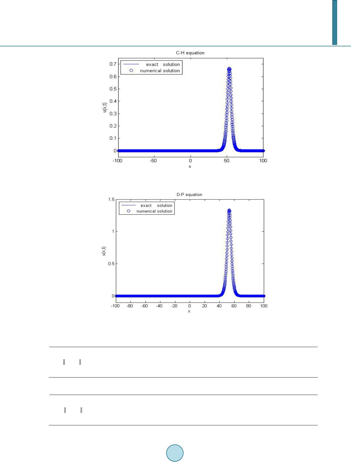

Z. Q. Xing et al.
985
Figure 1. Numerical simulations of the travelling wave solution (15) with
1k=
when
1000N=
0.1h=
,
20t=
.
Figure 2. Numerical simulations of the travelling wave solution (15) with
2 k=
when
1000N=
0.1h=
,
10t=
.
Table 1. When
1t=
;
1k=
, Convergence rate for the particle method.
x∆
0.1 0.05 0.025 0.0125 0.00625
exact
uu−
6.80e−03 1.70e−03 4.22e−04 1.06e−04 2.62e−05
Rate 2.00 2.01 1.96 2.01
Table 2. When
1t=
;
2 k=
, Convergence rate for the particle method.
x∆
0.1 0.05 0.025 0.0125 0.00625
exact
uu−
0.0306 7.60e−03 1.90e−03 4.76e−04 1.19e−04
Rate 2.01 2.00 2.01 2.00

Z. Q. Xing et al.
986
4. Conclusion
In this paper, we established the mathematical theory of the Lagrangian dynamics for the b-equation with a spe-
cial choice of the convolution kernel
G
and under a suitable class of initial data. To a numerical implementa-
tion of the method, it can be approximated by uniformly distributing particles. In the end, we obtained the nu-
merical solution though examples and specific data.
Acknowledgements
This work was supported by NSFC11171054.
References
[1] Camassa, R., Huang, J. and Lee, L. (2006) Integral and Integrable Algorithms for a Nonlinear Shallow-Water Wave
Equation. Journal of Computational Physics, 216, 547-572. http://dx.doi.org/10.1016/j.jcp.2005.12.013
[2] Chertock, A., Du Toit, P. and Marsden, J. (2012) Integration of the EPDiff Equation by Particle Methods. ESAIM:
Mathematical Modelling and Numerical Analysis, 46, 515-534. http://dx.doi.org/10.1051/m2an/2011054
[3] Chertock, A., L iu, J.G. and Pendleton, T. (2014) Elastic Collisions among Peakon Solutions for the Camassa-Holm
Equation. Applied Numerical Mathematics, in press. http://dx.doi.org/10.1016/j.apnum.2014.01.001
[4] Matsuo, T. and Miyatake, Y. (2012) Conservative Finite Difference Schemes for Degasperis-Procesi Equation. Journal
of Computational and Applied Mathematics, 236, 3728-3740. http://dx.doi.org/10.1016/j.cam.2011.09.004
[5] Camassa, R. and Lee, L. (2007) A Completely Integrable Particle Method for a Nonlinear Shallow-Water Wave Equa-
tion in Periodic Domains. Syst. Ser. A Math. Anal, 14, 1-5.
[6] Chertock, A., L iu, J. G. and Pendleton, T. (2012) Convergence of a Particle Method and Global Weak Solutions of a
Family of Evolutionary PDEs. SIAM Journal on Numerical Analysis, 50, 1-21. http://dx.doi.org/10.1137/110831386
[7] Camassa, R., Huang, J. and Lee, L. (2005) On a Completely Integrable Numerical Scheme for a Nonlinear Shallow-
Water Wave Equation. Journal of Nonlinear Mathematical Physics, 12, 146-162.
http://dx.doi.org/10.2991/jnmp.2005.12.s1.13
[8] Holden, H. and Raynaud, X. (2006) Convergence of a Finite Difference Scheme for the Camassa-Holm Equation.
SIAM Journal on Numerical Analysis, 44, 1655-1680. http://dx.doi.org/10.1137/040611975