Journal of Electromagnetic Analysis and Applications
Vol.06 No.10(2014), Article ID:50041,5 pages
10.4236/jemaa.2014.610030
The Exact Formulation of the Inverse of the Tridiagonal Matrix for Solving the 1D Poisson Equation with the Finite Difference Method
Serigne Bira Gueye
Département de Physique, Faculté des Sciences et Techniques, Université Cheikh Anta Diop, Dakar-Fann, Sénégal
Email: sbiragy@gmail.com
Copyright © 2014 by author and Scientific Research Publishing Inc.
This work is licensed under the Creative Commons Attribution International License (CC BY).
http://creativecommons.org/licenses/by/4.0/


Received 21 June 2014; revised 15 July 2014; accepted 8 August 2014
ABSTRACT
A new method for solving the 1D Poisson equation is presented using the finite difference method. This method is based on the exact formulation of the inverse of the tridiagonal matrix associated with the Laplacian. This is the first time that the inverse of this remarkable matrix is determined directly and exactly. Thus, solving 1D Poisson equation becomes very accurate and extremely fast. This method is a very important tool for physics and engineering where the Poisson equation appears very often in the description of certain phenomena.
Keywords:
1D Poisson Equation, Finite Difference Method, Tridiagonal Matrix Inversion, Thomas Algorithm, Gaussian Elimination, Potential Problem

1. Introduction
The finite difference method is a very useful tool for discretizing and solving numerically a differential equation. It is effectively a classical method of approximation based on Taylor series expansions that has help during the last years theoretical results to gain in accuracy, stability and convergence.
In fact, this method is very useful for solving for example Poisson equation. This elliptic equation appears very often in mathematics, physics, chemistry, biology and engineering. In one dimension, the resolution leads to a tridiagonal matrix in the case of centered difference approximation. This matrix, which is diagonally dominant, can be inverted with methods such as Gauss elimination, Thomas Algorithm Method [1] . These technics are powerful and very efficient.
We proposed here, a new and direct method of inversion of this tridiagonal matrix independently of the right- hand side. For Dirichlet-Dirichlet boundary problems, this innovative method is faster than the Thomas Algorithm. It gives better accuracy and is far more economical in terms of memory occupation.
First, the finite difference method is presented for the 1D Poisson equation. Secondly, the properties of the matrix associated with the Laplacian and its inverse are discussed. Then, the inverse matrix is determined and its properties are analyzed. Thus, verification is done considering an interesting potential problem, and the sensibility of the method is quantified.
2. Finite Difference Method and 1D Poisson Equation
We consider a function  which satisfies the Poisson equation
 , in the interval
 , where
  is a specified function.
  fulfills the Dirichlet-Dirichlet boundary conditions
 ![]() and
and![]() . We consider an one-dimensional mesh with
. We consider an one-dimensional mesh with ![]() discrete points
discrete points![]() . Each point
. Each point ![]() is de-
is de-
fined by![]() , where
, where ![]() being the step size. We define
being the step size. We define![]() ,
, ![]() ,
,![]() .
.
We have chosen the centered difference approximation , in this work, for the fact that it gives a tridiagonal, diagonally dominant, and symmetric matrix. Considering all the above mentioned criteria, one can rewrite the 1D Poisson equation in a set of algebraic equations:
 (1)
(1)
One gets a linear system of  equations, which can be written in a matrix form [2]
 (2)
(2)
Thus, solving the 1D Poisson equation means to invert the negative definite, and regular  -matrix
 . Its inverse, that we noted
 , is also symmetric. Both matrices have the following properties:
 (3)
(3)
and
 (4)
(4)
where  is the Kronecker’s delta.
3. The Inverse of Matrix 
From (4), we derive successively the following interesting relations:
 (5)
(5)
with (5), one sees that the matrix  is entirely determined if the term
  is known. This term can be determined by observing the behavior of
  for different
  values: It holds
 (6)
(6)
From (5) and (6), we get
 (7)
(7)
Now, the matrix  is completely and exactly determined.
  with
with
 (8)
(8)

The solution of the 1D Poisson equation is obtained with a simple, extremely fast matrix multiplication: . Thus, the numerical resolution of the 1D Poisson equation which is an interesting topic in physics and engineering is made easy and very accurate.
Analysis
A first analysis of the matrix  let us believe that, this new method possesses an algorithm complexity of
 , which is situated between the Gauss eliminations
  and the one of Thomas’s
  [1] .
[1] .
A deeper analysis of the matrix  shows that the complexity brought by the Thomas method is largely improved in this study. In addition, one can see a close link between its row vectors and column vectors.
The matrix  is also persymmetric:

All the information about it, can be found in the upper triangle (in gray color, see Figure 1).
Further, we can even find very interesting relations in this matrix which can help refining the final solution.
That is what we effectively did, and one can see a direct solution for  at the point
 , which can be expressed by
 (9)
(9)
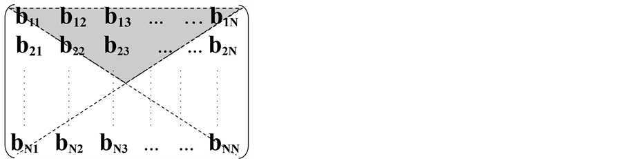
Figure 1. Matrix symmetries.
Also a direct solution for  at the point
  is:
is:
 (10)
(10)
Generally, a very important recurrence relation can be obtained, which gives all solutions:
 (11)
(11)
which is equivalent to:
 (12)
(12)
This very innovative Equation (12) gives directly and accurately all the solution that we are looking for. It proves that our method is direct, faster than the one of Thomas’s in this context and gives as well better accuracy. Furthermore, it is far more economical in terms of memory occupation. This is due to the fact that the matrix  does not necessitate to be generated. A programmer does not need to declare nor to define the matrix
  in his code.
In conclusion to this, we can say that the matrix  is the key of this efficient new method. This matrix
 , which is the inverse of matrix
 , is determined explicitly, directly, and independently of the right-hand side of the Poisson equation.
N.B.: One can prove using mathematical induction that . It holds for the
  cofactor of
 :
: . We call the matrix
  Bira’s Matrix.
4. Verification with a Potential Problem
We consider a scalar potential , defined in [0, 1], which satisfies
 .
.  fulfills the following boundary conditions:
 . The exact solution is
 (13)
(13)
With the finite difference method, we take ,
,  ,
,  ,
,  , and
, and . The solution is
 (14)
(14)
Discussions
We define the variable , which is the relative error at point
  for
for .
.  represents
 .
.
Generally, we have
 (15)
(15)
We can also define the average value of the relative error for a given :
: . For
. For , it is:
 .
.
We obtain the following results, presented in Table 1.
The table shows that the solution is very accurate. Notwithstanding that we have been interested in determining the sensibility of the proposed method. Effectively, we have plotted  for different
  values.
We obtain a hyperbola, which can be predicted as proportional to .
.
This curve is fitted with a function which can be defined as
 (16)
(16)
where . We obtain two curves represented in Figure 2.

Table 1. Results and relative error.
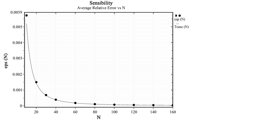
Figure 2. Sensibility.
We realize that the average relative error  behaves like a truncation error that we express in the fol-
lowing manner .
. ![]() is the fourth order derivative of the
is the fourth order derivative of the ![]() function in a point (here
function in a point (here![]() ) which belongs to the interval
) which belongs to the interval![]() .
.
For our given function ![]() and also the results from the fitting, we have the following relations [3] :
and also the results from the fitting, we have the following relations [3] :
![]() (17)
(17)
This proves that the method is very accurate, naturally stable, robust, quick and precise.
5. Conclusions
This paper has provided a new improved method for solving the 1D Poisson equation with the finite difference
method. Accurate results have been obtained with a sensibility found to be as the function of![]() . In fact, the inverse of the tridiagonal matrix, which is associated with this differential equation, is determined directly, exactly, and independently to the right-hand side. Thus, a new formulation of the solution is given with an algorithmic complexity of O(N). With this innovative method, the 1D Poisson equation, with Dirichlet-Dirichlet boundary condition is solved, with only one programming loop. This new approach provides also gain in accuracy and economy in memory allocation.
. In fact, the inverse of the tridiagonal matrix, which is associated with this differential equation, is determined directly, exactly, and independently to the right-hand side. Thus, a new formulation of the solution is given with an algorithmic complexity of O(N). With this innovative method, the 1D Poisson equation, with Dirichlet-Dirichlet boundary condition is solved, with only one programming loop. This new approach provides also gain in accuracy and economy in memory allocation.
A future work can consider Neumann or mixed boundary conditions.
Acknowledgements
I would like to thank my colleagues Dr. Cheikh Mbow and Dr. Kharouna Talla for benefit discussions and remarks that contribute to improving the quality of this paper.
References
- Conte, S.D. and de Boor, C. (1981) Elementary Numerical Analysis: An Algorithmic Approach. 3rd Edition, McGraw- Hill, New York, 153-157.
- Leveque, R.J.E. (2007) Finite Difference Method for Ordinary and Partial Differential Equations, Steady State and Time Dependent Problems. SIAM, 15-16. http://dx.doi.org/10.1137/1.9780898717839
- Mathews, J.H. and Kurtis, K.F. (2004) Numerical Methods Using Matlab. 4th Edition, Prentice Hall, Upper Saddle River, 323-325, 339-342.