Int'l J. of Communications, Network and System Sciences
Vol.6 No.12(2013), Article ID:41061,6 pages DOI:10.4236/ijcns.2013.612055
Adaptation in Stochastic Dynamic Systems—Survey and New Results IV: Seeking Minimum of API in Parameters of Data
School of Mathematics and Information Technology, Ulyanovsk State University, Ulyanovsk, Russia
Email: kentvsem@gmail.com, tsyganovajv@gmail.com
Copyright © 2013 Innokentiy V. Semushin, Julia V. Tsyganova. This is an open access article distributed under the Creative Commons Attribution License, which permits unrestricted use, distribution, and reproduction in any medium, provided the original work is properly cited.
Received October 9, 2013; revised November 9, 2013; accepted November 16, 2013
Keywords: Linear Stochastic Systems; Parameter Estimation; Model Identification; Identification for Control; Adaptive Control MSC (2010); 93E10; 93E12; 93E35
ABSTRACT
This paper investigates the problem of seeking minimum of API (Auxiliary Performance Index) in parameters of Data Model instead of parameters of Adaptive Filter in order to avoid the phenomenon of over parameterization. This problem was stated by Semushin in [2]. The solution to the problem can be considered as the development of API approach to parameter identification in stochastic dynamic systems.
1. Introduction
The recent papers [1,2] gave a survey of the field of adaptation in stochastic systems as it has developed over the last four decades. The author’s research in this field was summarized and a novel solution for fitting an adaptive model in state space (instead of response space) was given.
In this paper, we further develop the Active Principle of Adaptation for linear time-invariant state-space stochastic MIMO filter systems included into the feedback or considered independently.
We solve the problem of seeking minimum of Auxiliary Performance Index (API) in parameters of Data Source Model (DSM) instead of parameters of Adaptive Filter (AF) in order to avoid difficulties known as Phenomenon of Over Parameterization (PhOP). The PhOP means that the number of parameters to be adjusted in AF is usually much greater than that in DSM. The solution of this problem will enable identification in the space of lower dimension and at the same time provide estimates of the given system state vector according to Original Performance Index (OPI). We verify the obtained theoretical results by two numerical simulation examples.
2. Parameterized Data Models 
Following the previous results of [1,2], we assume that all data models  forming a set
  are parameterized by an
  -component vector
 . Each particular value of
  (which does not depend on time) specifies a
 . Hence
 (1)
(1)
where  is the compact subset of
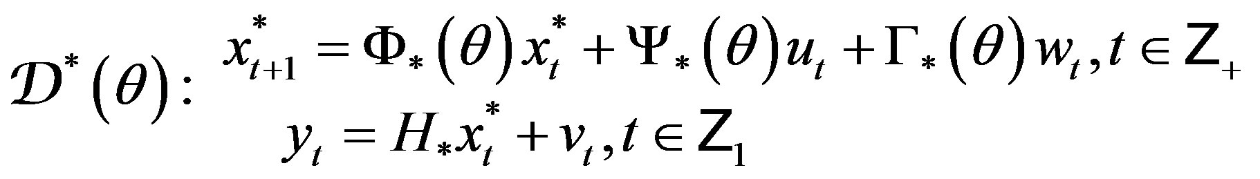
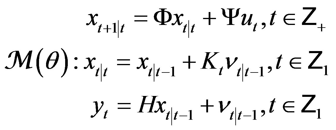
 . A given physical data model (PhDM) is described by the following equations:
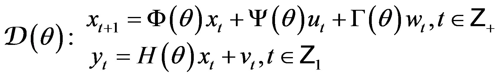 (2)
(2)
where  denotes nonnegative integers,
  strictly positive integers, and
  all integers.
Every model  (2) is assumed to be acting between adjacent switches as long as it is sufficient for accepting as correct the basic theoretical statement (BTS) that all processes related to the
  are wide-sense stationary. This statement amounts to the following assumptions. The random
  with
with  is orthogonal [3] to
  and
and , the zero-mean mutually orthogonal wide-sense stationary orthogonal sequences with
  and
and  for all
 ;
;  is orthogonal to
  and
and  for all
 ;
;  is a given signal; it is an “external input” when considering the open-loop case or a control strategy function
 (3)
(3)
when considering the closed-loop setup.
Stackable vectors of previous values
 (4)
(4)
constitute the experimental condition  (cf. Ljung [4]).
By assumption,  is generated by the completely observable PhDM (2), so we can move from the physical state variables
  in (2) to another
  through the similarity transformation
 . Such transformation uniquely determines a new state representation
 (5)
(5)
of the standard observable data model (SODM) (cf. Semushin [2]).
For convenience in the below we shall omit the subscript  for all the matrices describing PhDM or SODM.
3. Parameterized Innovations
As before, the above data model of a time-invariant data source will be referred to as the conventional model, no matter whether it is PhDM (2) or SODM (5). Here we use another innovation model, that differs from the timeinvariant (due to BTS) innovation model, presented in [2]:
 (6)
(6)
with , the initial
 , and
, and which is the well-known (not necessarily steady-state) Kalman filter with the innovation process
 , the optimal state predictor
 , the gain
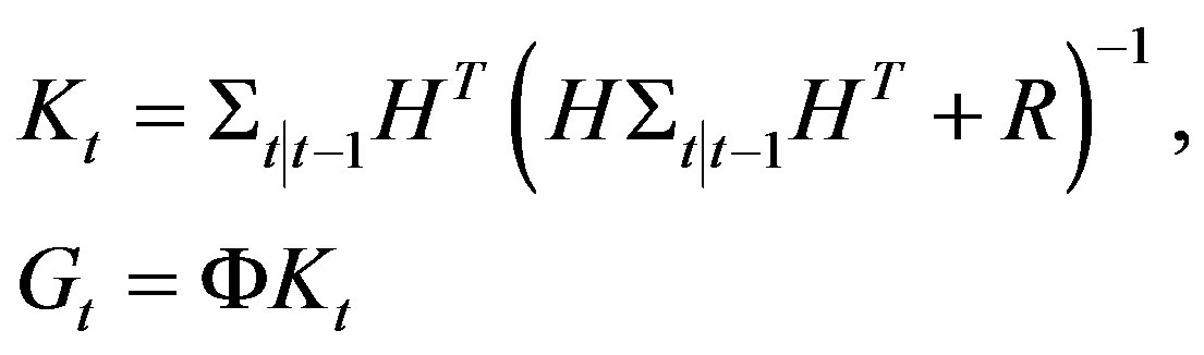 (7)
(7)
and  satisfying the discrete Riccati iterations [5]
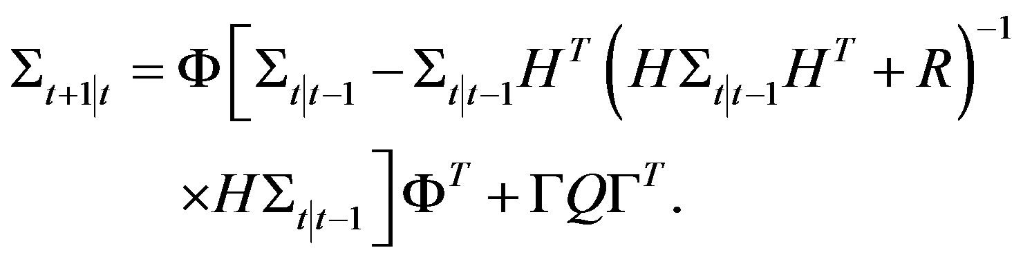 (8)
(8)
Concurrently, another form
 (9)
(9)
with the initial , which is equivalent to (6), can be used where
  is the optimal “filtered” estimator for
  based on experimental condition
  (4). When
  ranges (or switches) over
  as in (1), we obtain the set of Kalman filters
 (10)
(10)
We consider the mean-square criterion
 (11)
(11)
defined for a one-step predictor  through its error
  in the Kalman filter. Thus in the basis forming the state-space,
  (9) is the model minimizing the Original Performance Index (OPI)
  (11) at any
 , which is large enough for BTS to hold, so that writing
  or
or  as well as any other finitely shifted time in (11) makes no difference.
4. Uncertainty Parameterization
In contrast to our previous work [2], we do not consider the four levels of uncertainty. Assume that system (2) (and also the SODM (5)) is parameterized by an  - component vector
  of unknown system parameters, which needs to be identified. This means that the entries of the matrices
 ,
,  ,
,  ,
,  ,
,  ,
,  are functions of
 . However, for the sake of simplicity we will supress the corresponding notations below, i.e. instead of
 ,
,  ,
,  ,
,  ,
,  ,
,  we will write
 ,
,  ,
,  ,
,  ,
,  ,
, . We make the same assumptions about the SODM.
5. The Set  of Adaptive Models
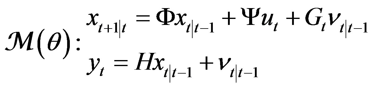
Let us consider the set of adaptive models
 (12)
(12)
Here we emphasize the fact that we construct adaptive models in the same class as  belongs to with the only difference that the unknown parameter
  in
in  is replaced by
  to obtain
 . In so doing, each particular value of
 , an estimate of
 , leads to a fixed model
 . In accordance with The Active Principle of Adaptation (APA) [1], only when
  ranges over
  in search of
  for the goal
  or
or  as governed by a smart, unsupervised helmsman equipped by a vision of the goal in state space and able to pursue it, we obtain a model
  of active type within the set
  (12). In this case,
  will act as a self-tuned model parameter and so should be labeled by
 , the time instant of model’s inner clock, in order to get thereby the emphasized notations
  and
and  in describing parameter identification algorithms (PIAs) to be developed. From this point on
  becomes an adaptive estimator.
Remark 1 Note in passing that pace of  may differ from that of
 . We shall need to discriminate between
  and
and  later when developing a PIA.
Remark 2 If we work in the context of SODM, the set
 (13)
(13)
instead of (12) should be used.
At this junction, we identify the following tasks as pending:
1) Express  or
or  in an explicit form.
2) Build up APIs that could offer vision of the goal.
3) Examine APIs’ capacity to visualize the goal.
4) Develop a PIA that could help pursuing the goal.
Consider here the first three points consecutively.
5.1. Parameterized Adaptive Models
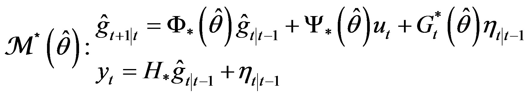
Reasoning from (6), (9), we set the adaptive model
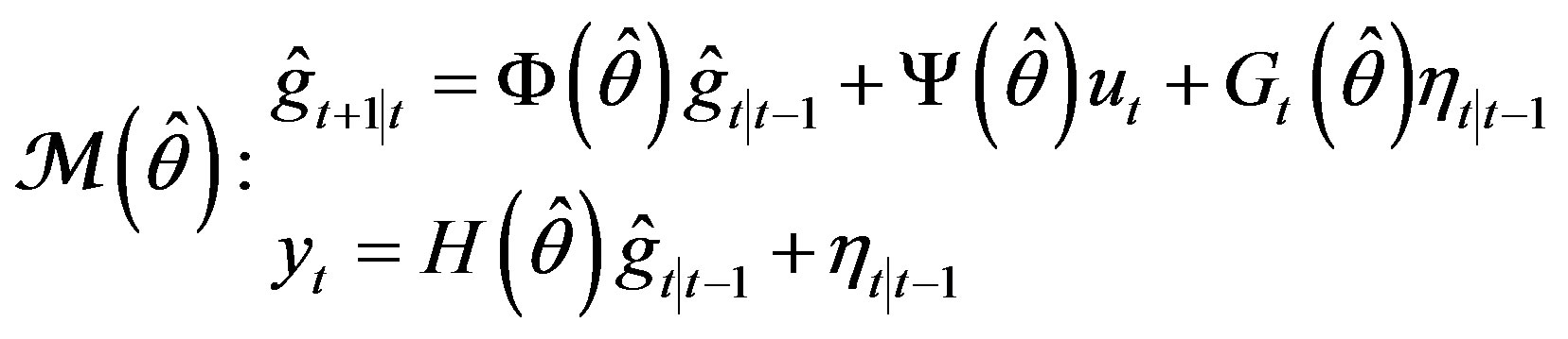 (14)
(14)
or equivalently (due to ) the model
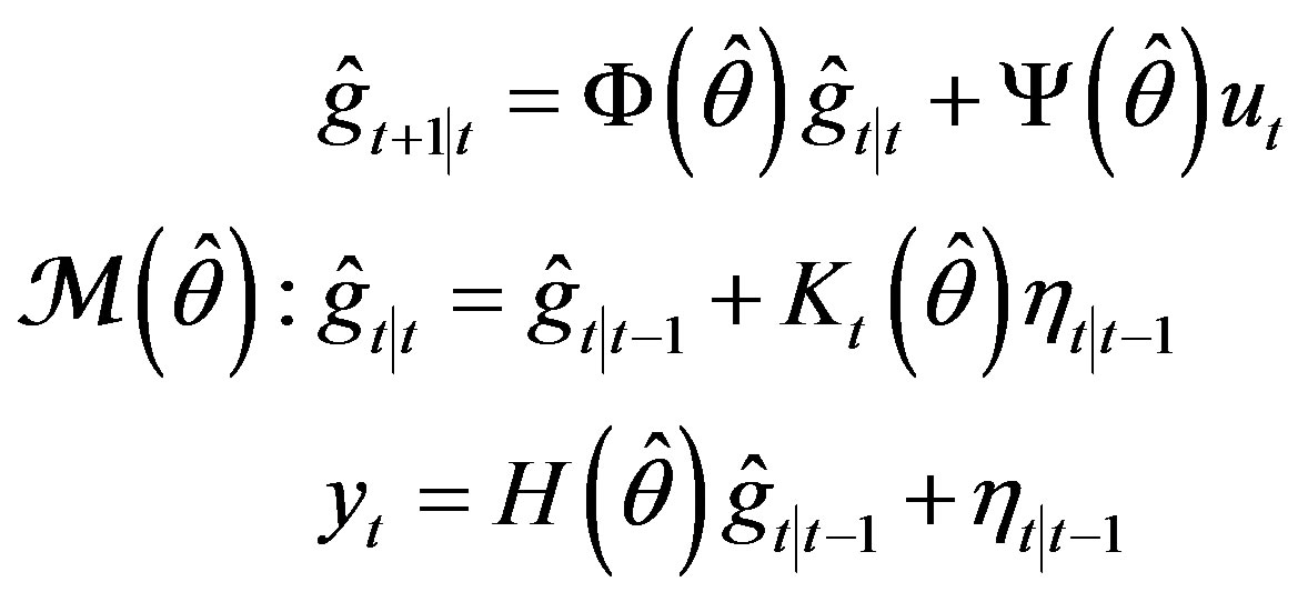 (15)
(15)
as a member of  (12). Here
  is the self-tuned parameter intended to estimate (in one-to-one corresponddence) parameter θ. In parallel, reasoning from
 , we build the adaptive model
 (16)
(16)
or equivalently (due to ) the model
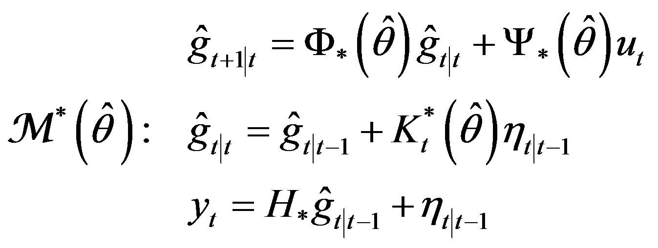 (17)
(17)
where  does not depend on
 . Matrices
and  are evaluated according to (7), (8).
Adaptor  using (14)-(15) (or alternatively,
  using (16)-(17)) is supposed to contain a PIA to offer the prospect of convergence. For convergence in parameter space, we anticipate almost surely (a. s.) convergence, as it is the case for MPE identification methods [3,4]. It actuates either or both of the two other types of convergence. The type of convergence in state space, as well as in response space, is induced by the type of Proximity Criterion, PC (cf. [2], Figures 1-3). As seen from (11), we are oriented to the PC, which is quadratic in error; this being so, it would appear reasonable that these convergences would be in mean square (m. s.). Thus we anticipate the following properties of our estimators:
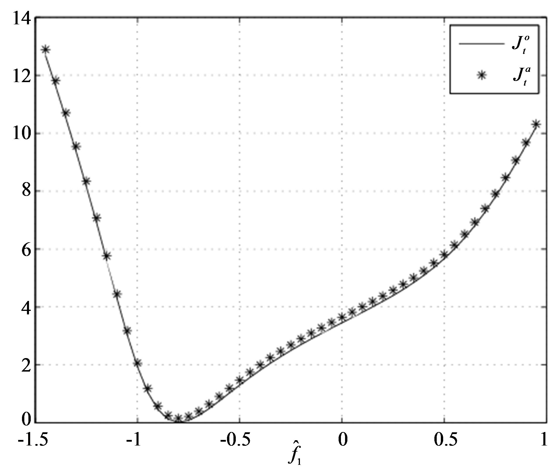
Figure 1. The values of  and
and  versus the estimates of parameter
  (Example E1).
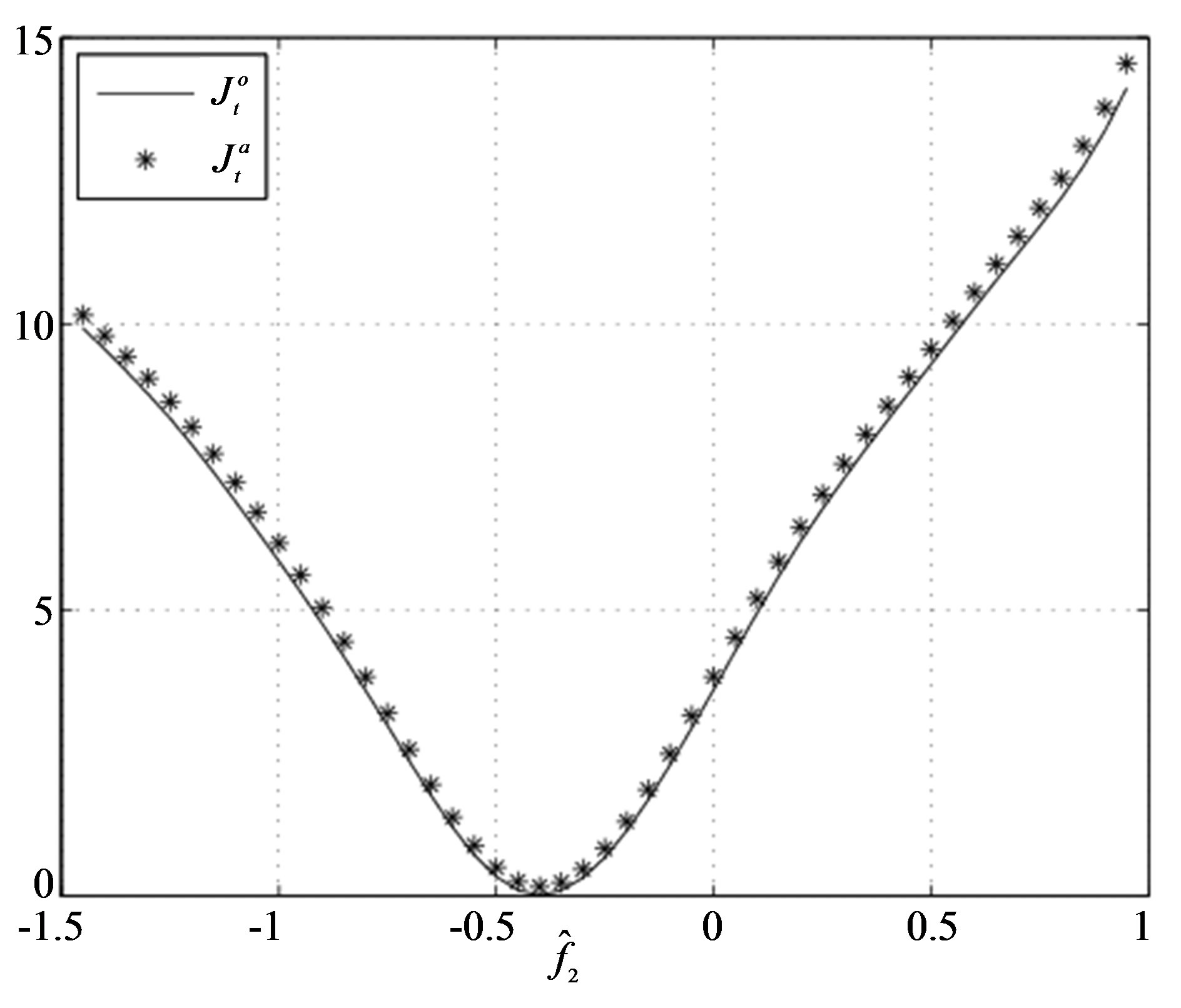
Figure 2. The values of  and
and  versus the estimates of parameter
  (Example E1).
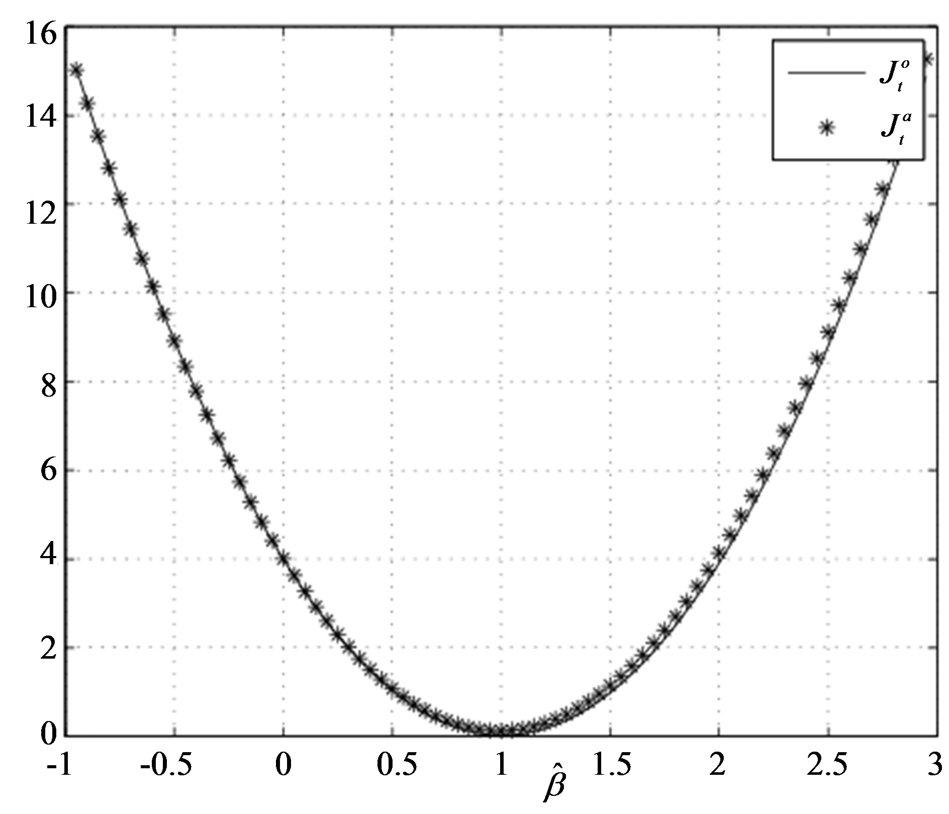
Figure 3. The values of  and
and  versus the estimates of parameter β (Example E1).
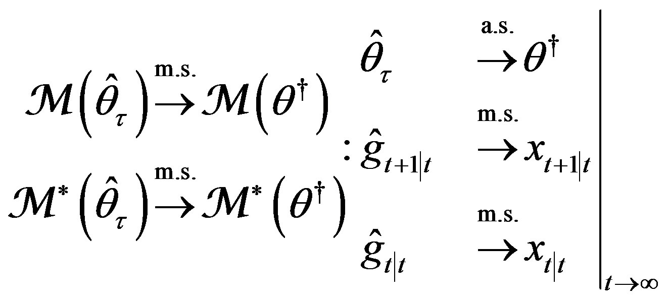 (18)
(18)
With the understanding that errors for PC
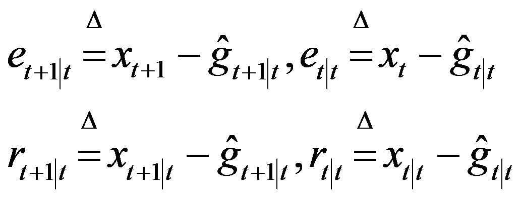 (19)
(19)
are fundamentally invisible for any measurement, we search for a function
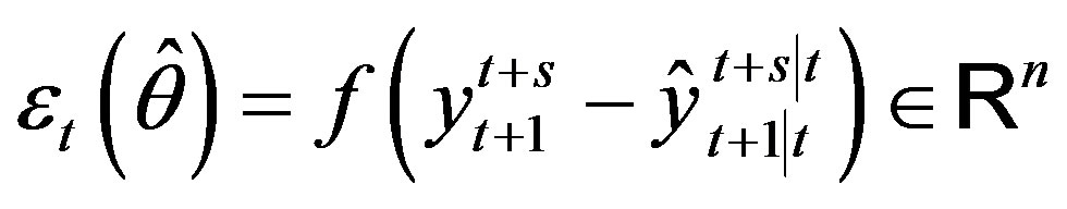 (20)
(20)
of the difference in two terms: outputs  generated by Data Source described in any appropriate form (2), (5)(6), or (9), and their estimates
  generated by the adaptive model
  (or
(or ). For
  in
in
(20), we will also use notations  or
or , thus bringing them into correlation with
  or
or  (correspondingly, with
  or
or ) from (19). Then
 (21)
(21)
will be taken as the PC and determined with the key aim:
True (Unbiased) System Identifiability
Here, the equivalence symbol  needs clarification. Its sense correlates with the above concept of convergence (18). Necessary refinements will be done (in Theorem 1).
5.2. API Identifiability of 
Let the auxiliary process (20) be built for the API (21) as
 (22)
(22)
or, equivalently, as
 (23)
(23)
where special matrix transformations are used (see the section “Ancillary Matrix Transformations” of [2]).
Theorem 1 Let  (20) be a vector-valued ncomponent function of
 . If
. If  is defined by
(22) or (equivalently) (23) in order to form the API (21), then minimum in  of the API fixed out at any instant t is the necessary and sufficient condition for adaptive model
  to be consistent estimator of
  in mean square,
 , that is True (Unbiased) m.s. System Identifiability
in the following three setups:
Setup 1 (Random Control Input)  is a preassigned zero-mean orthogonal wide-sence stationary process orthogonal to
  but in contrast to
  and
and , known and serving as a testing signal;
Setup 2 (Pure Filtering) , and Setup 3 (Close-loop Control) with
 , which does not depend on
 .
.
Proof is similar to the proof of Theorem 2 in [2].
Remark 3 Our main goal is to identify the vector  of unknown parameters. The minimization of API by some PIA allows us to determine the optimal value
 . Then it must be substituted into (14)-(15) (or (16)-(17))
to get the optimal model  (or
(or ). At the same time, we obtain the optimal estimates
  (or
(or ) according to OPI.
5.3. Main Conceptual Novelty
Seeking minimum of API in parameters of Data Model instead of parameters of Adaptive Filter is more profitable, as:
• It takes into account the dynamics of the discrete Riccati equations, which positively affects the quality of parameter and state vector estimates.
• The number of unknown parameters can be substantially (an order of magnitude or more) reduced thus helping avoid the difficulties of PhOP.
• API gradient is calculated easily—without the construction of sensitivity model of adaptive filter.
• It can be implemented in the case of non-stationary systems, which is critical, for example, to handle the navigation data.
Thus, the proposed variant of API method is a new, thanks to the solution of its important tasks:
1) Numerical construction of API, which has the same minimizing argument that the OPI does;
2) The numerical minimization of the API by conventional optimization methods such as Newton-Raphson method, and 3) The combination of parameter identification of the system with the process of adaptive estimation of its states.
6. Simulation Examples
We take two examples to simulate:
E1 Second order open-loop system with unknown parameters  is given by
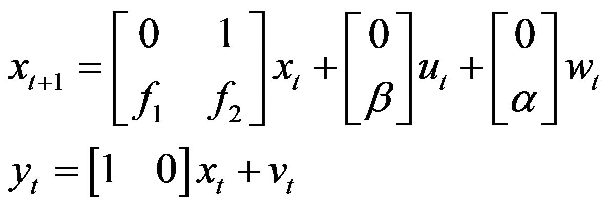
Unknown parameters should be identified. Adaptive model parameter is the four-component vector
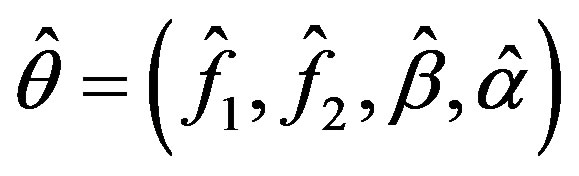 .
.
Its true value is
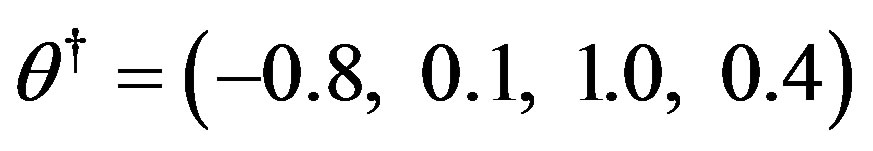 .
.
Covariances  and
and  of the noises
  and
and  are equal to 0.04 and 0.06, correspondingly.
E2 The same (but closed-loop) system as in E1. The system is designed to operate with a minimum expected control cost
Unknown parameters ,
,  ,
,  and
and  should be identified. The true values of parameters are the same as in E1.
Simulation results of Figures 1-4 and 5-7 obtained from Julia Tsyganova’s MATLAB programs demonstrate equimodality (coincidence of the minimizing arguments) of the auxiliary performance index with the original performance index. It is seen that the minimums of OPI and API coincide near . Thus, the obtained results confirm applicability of the presented method.
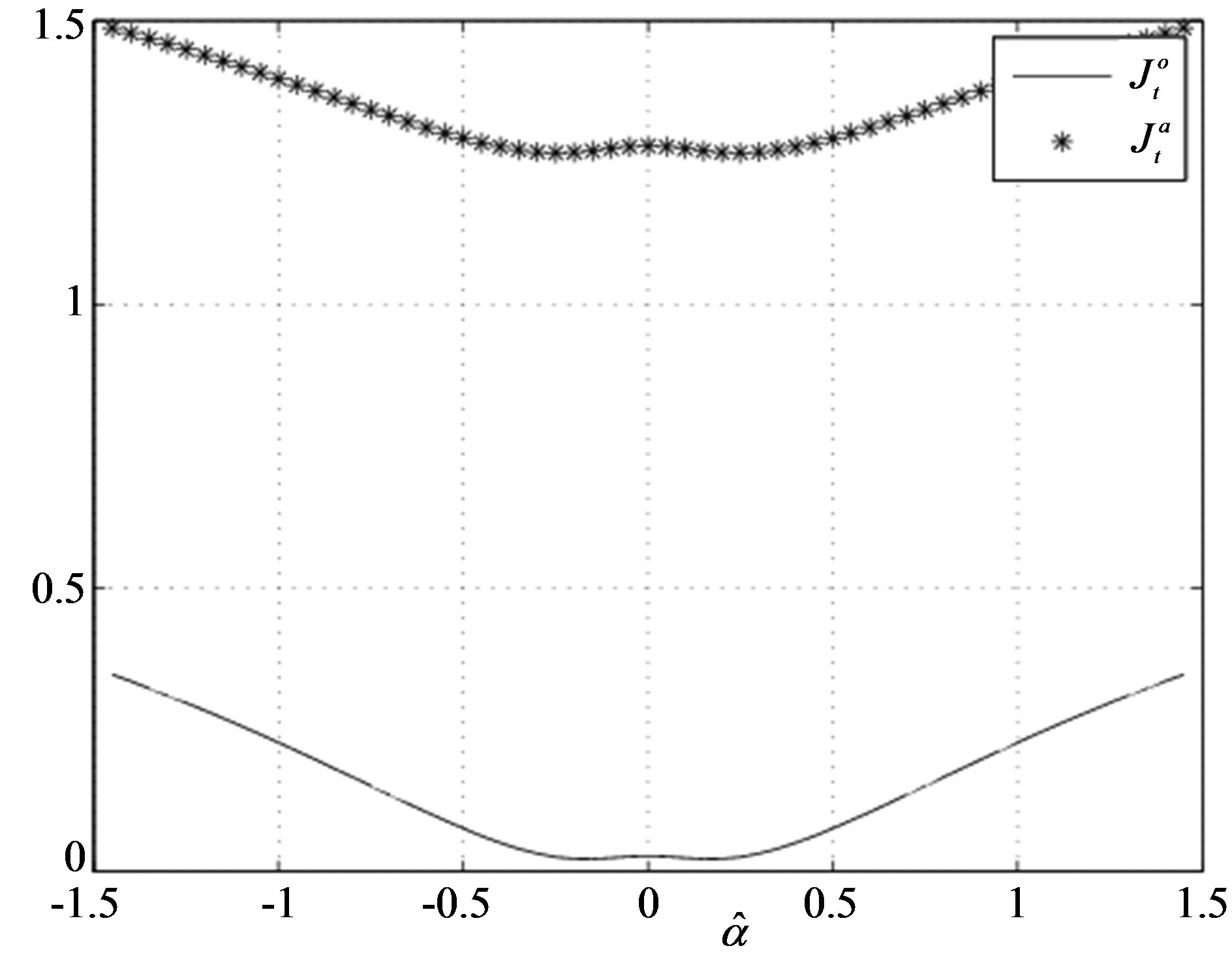
Figure 4. The values of  and
and  versus the estimates of parameter
  (Example E1).
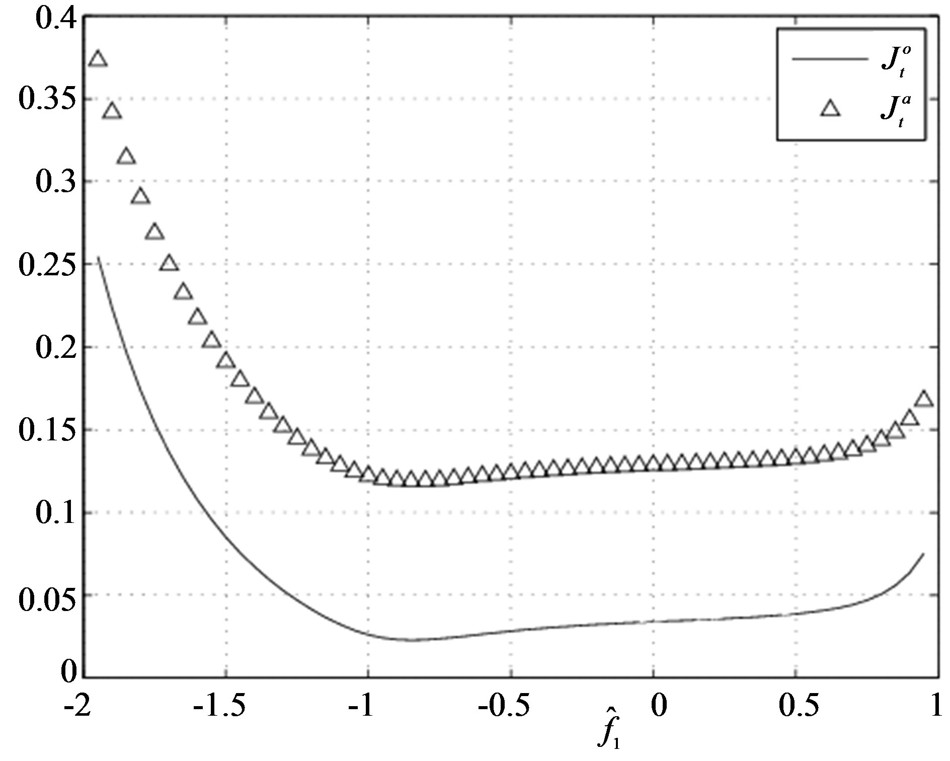
Figure 5. The values of  and
and  versus the estimates of parameter
  (Example E2).
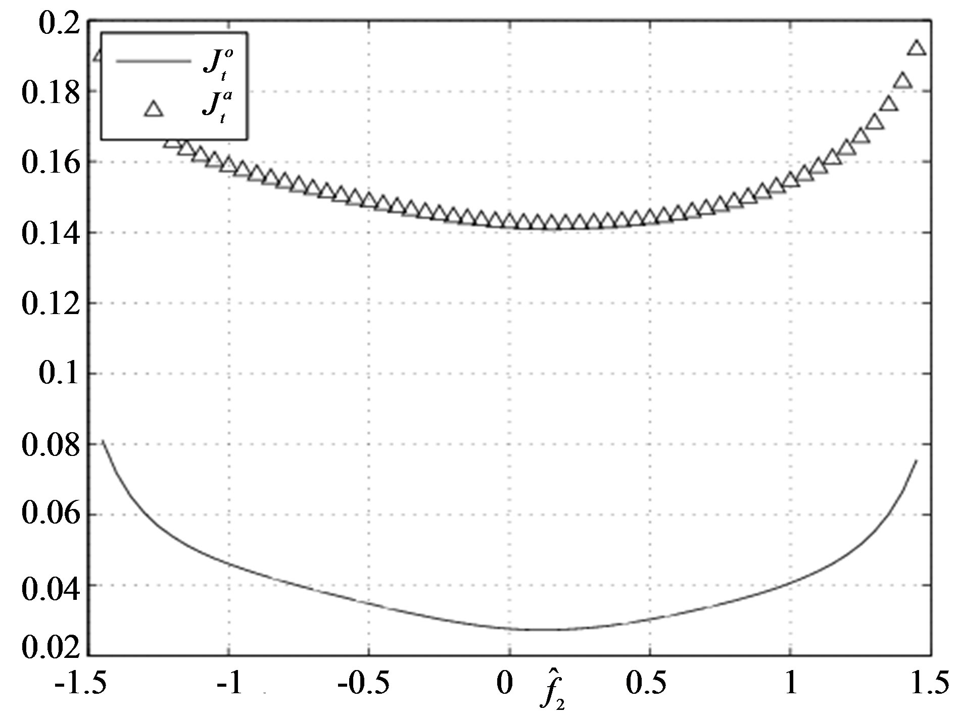
Figure 6. The values of  and
and  versus the estimates of parameter
  (Example E2).
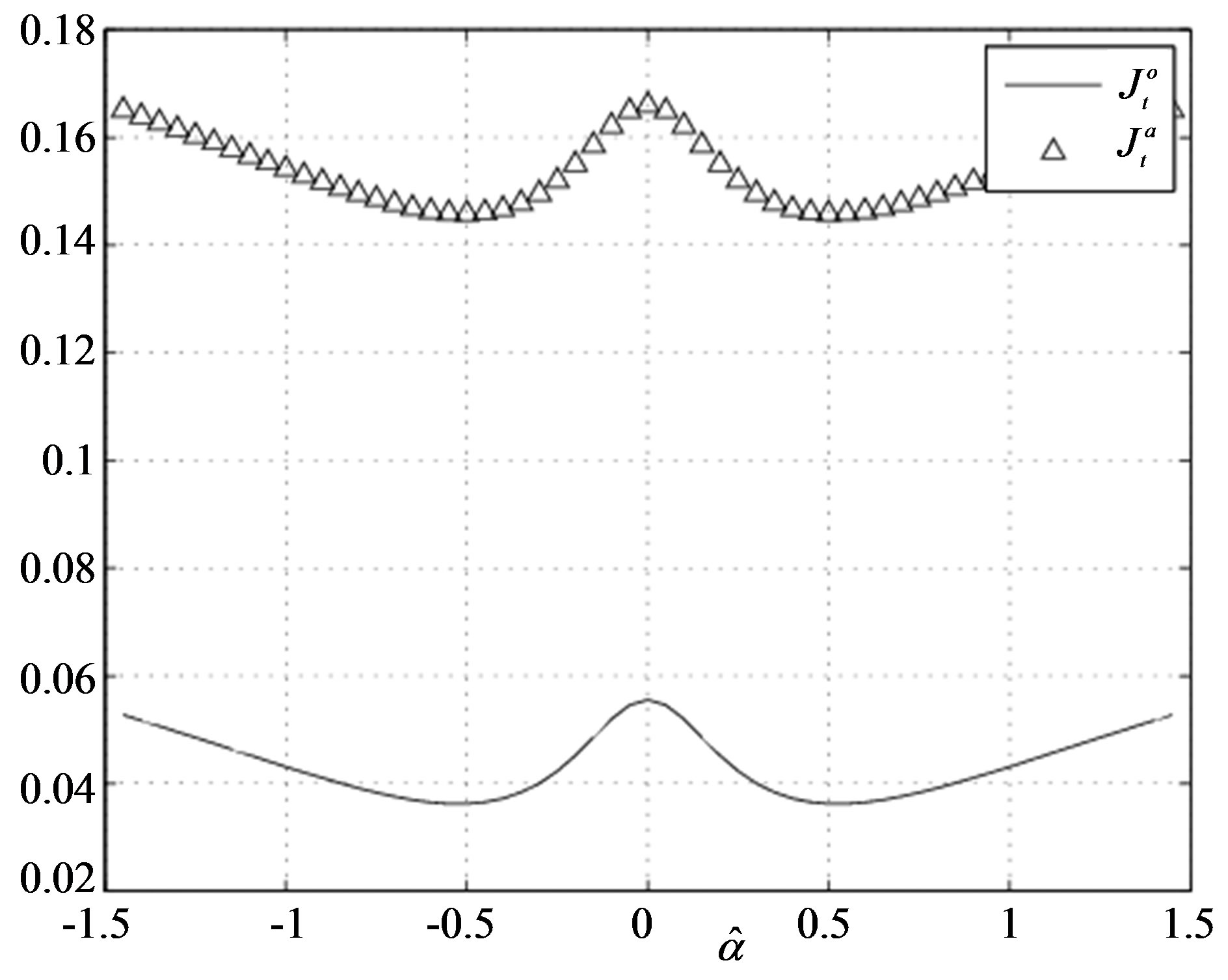
Figure 7. The values of  and
and  versus the estimates of parameter
  (Example E2).
7. Conclusion
The present paper gives a comprehensive solution to the problem of seeking minimum of  in parameters
 of Data Model
  or
or  instead of parameters of Adaptive Filter
  or
or . The obtained results were verified by two numerical simulation examples.
Our further research is aimed at obtaining solutions to the following issues:
• Economic feasibility, numeric stability and convergence reliability of each proposed parameter identification algorithm.
• Numerical testing of the approach and determining the scope of its appropriate use in real life problems, for example, in Health Care field [6].
8. Acknowledgements
This work was partly supported by the RFBR Grant No. 13-01-97035.
REFERENCES
- I. V. Semushin, “Adaptation in Stochastic Dynamic Systems—Survey and New Results I,” International Journal of Communications, Network and System Sciences, Vol. 4, No. 1, 2011, pp. 17-23. http://dx.doi.org/10.4236/ijcns.2011.41002
- I. V. Semushin, “Adaptation in Stochastic Dynamic Systems—Survey and New Results II,” International Journal of Communications, Network and System Sciences, Vol. 4, No. 4, 2011, pp. 266-285. http://dx.doi.org/10.4236/ijcns.2011.44032
- P. E. Caines, “Linear Stochastic Systems,” John Wiley and Sons, Inc., New York, 1988.
- L. Ljung, “Convergence Analysis of Parametric Identification Methods,” IEEE Transactions on Automatic Control, Vol. 23, No. 5, 1978, pp. 770-783. http://dx.doi.org/10.1109/TAC.1978.1101840
- E. Mosca, “Optimal, Predictive, and Adaptive Control,” Prentice Hall, Inc., Englewood Cliffs, 1995.
- I. V. Semushin, J. V. Tsyganova and A. G. Skovikov, “Identification of a Simple Homeostasis Stochastic Model Based on Active Principle of Adaptation,” Book of Abstracts Applied Stochastic Models and Data Analysis ASMDA 2013 & Demographics, Barcelona, 25-28 June 2013, p. 191.