Journal of Water Resource and Protection
Vol.5 No.8A(2013), Article ID:35685,7 pages DOI:10.4236/jwarp.2013.58A005
Small Water Distribution System Operations and Disinfection By Product Fate
Department of Civil and Environmental Engineering, University of Missouri-Columbia, Columbia, USA
Email: *srp352@mail.missouri.edu
Copyright © 2013 Sandhya Rao Poleneni, Enos C. Inniss. This is an open access article distributed under the Creative Commons Attribution License, which permits unrestricted use, distribution, and reproduction in any medium, provided the original work is properly cited.
Received May 29, 2013; revised July 1, 2013; accepted August 6, 2013
Keywords: Trihalomethanes; Pipe Loop; Chlorination; Distribution Systems; Formation Kinetics
ABSTRACT
The Stage-2 Disinfectant and Disinfection By-Product (D/DBP) regulations force water utilities to be more concerned with their finished and distributed water quality. Compliance requires changes to their current operational strategy, which affect the formation of DBPs over time. This study quantifies changes in DBP formation and chlorine decay kinetics under different operational conditions and pipe materials found at many small-scale water utilities. A physical model (Pipe Loop) of a distribution system was used to evaluate the change in water quality from conditions such as having a high chlorine dosage entering the distribution system, using a chlorine booster system in the distribution system, and operation of clearwells/storage tanks. The High Chlorine Run (HC) is least favorable option with approximately 64% and 30% higher TTHMs than Normal Run (NR) and Chlorine Booster Run (CB), respectively. High Chlorine conditions also minimize the wall effects. The location of Boosters should always be after the storage systems to avoid extra contact time that can produce approximately 23% - 78% higher TTHMs. The following trends are discovered from the data analysis: Chlorine residual HC > CB > NR and TTHM NR > CB > HC.
1. Introduction
Chlorination is one of the most widely used disinfection processes in water treatment plants because chlorine is a very effective disinfectant and is relatively easy to handle; the capital costs of installation are low; it is cost effective, simple to dose, measure and control; and, it has a reasonably prolonged residual [1-3]. Despite the benefits of chlorine, halogenated disinfection by-products (DBPs) are formed due to the interaction of aqueous free chlorine with natural organic matter (NOM), like humic substances, present in water [4,5]. Water utilities use different operational strategies to overcome physical (infrastructure, source water quality, distribution system layout etc.) and financial constraints to maintain consistent water quality throughout their distribution system and meet water demand of its customers. The selection of these strategies is mainly based on system-specific conditions and preferences of the utility operator. Many utilities use more than one strategy to ensure compliance with seasonal changes in source water quality and water demand [6]. With the Stage-II Disinfectants and Disinfectant ByProduct Rule regulation compliance date approaching, many small-scale utilities are adopting techniques to balance between protection against microbial risks and the risks posed by harmful by-products [7-9]. Typically, small-scale utilities are operated in one of the following ways: Normal conditions, High Chlorine conditions and Chlorine Booster conditions.
Since the exact chemical composition of organic matter is unknown, a number of kinetic models have been developed to approximate chlorine decay in bulk water [7-14]. First-order kinetic models with respect to chlorine are the most commonly used models [7,8,12,13,15]. They are known for their simplicity, wide range of applicability, and reasonable representation of chlorine decay in distribution systems [7,8,12,13]. The differential form of the decay model for the bulk fluid is shown in equation (1) [7,15].
 (1)
(1)
where, C = chlorine concentration in the bulk fluid (milligram/liter, mg/L); t = time (days or hours); and kb = bulk decay coefficient (day−1 or hour−1).
The first-order chlorine decay model reactions at the pipe wall are given by
 . (2)
. (2)
where, kw = wall decay coefficient (cm/day); rh = hydraulic radius (cm); and Cw = concentration of chlorine at the wall (mg/L), which is a function of bulk chlorine concentration [7,15]. The mass-transfer-based model of chlorine decay in distribution systems can be explained in terms of laminar and turbulent flow conditions. Studies have shown that when calculations are made under laminar flow conditions, the rate constant of wall reactions is nearly zero and there is no mass transfer with the pipe wall. However, in real distribution systems, the flow is generally turbulent and is directly proportional to flow velocity [16]. Therefore, various investigators have used data from Pipe Loop experiments or field data to calculate the wall decay coefficient (kw; equation (3)) as the difference between overall decay coefficient (kT) and bulk decay coefficient (kb) [7,15,16].
 (3)
(3)
Previous research and data from the loop built as part of this research has shown that Total Trihalomethanes (TTHM) formation and chlorine consumption have a strong linear relationship at a pH range between 6 and 8 while a fairly linear relationship exists at pH values above 8 [7,15,17]. This can be attributed to the fact that higher rates of chlorine consumption are observed with increases in pH. The linear relationship between TTHM formation and chlorine consumption can be represented as
 . (4)
. (4)
where, TTHM = total trihalomethane formation (microgram/liter, μg/L); Y = yield parameter (μg of TTHM formed/ mg of chlorine consumed) and M = intercept from linear regression analysis of experimental data [7, 8,18]. Yield depends on many factors including chemical composition and structure of the organic material in water, pH and temperature [7,18]. Equation (4) was used to calculate the TTHM yield in our research.
2. Methods
This research was conducted using a physical model of distribution system (Pipe Loop) built at Columbia Water Treatment Plant using 10.16 cm (4 in) PVC pipe [19]. In order to simulate a Normal Run (NR), finished water from the City of Columbia water treatment plant (chlorinated water before ammonia addition) is allowed to enter the Pipe Loop via the Water Tank attached to it (Figure 1). The water was recirculated in the looped system for 7 days with water samples collected at daily intervals. Collected samples were tested for free and total chlorine residual, total organic carbon (TOC), pH, UV254

Figure 1. Schematic of the pipe loop used in experiments to determine effects of distribution system management. Water tank shown was used to simulate clearwell.
and TTHM as a function of time over a period of 10 months.
The scenarios discussed in this paper are: Normal Run vs. High Chlorine Run, minimization of wall reactions, High Chlorine Run vs. Chlorine Booster Run, chlorinelimited conditions and location of placement of chlorine boosters.
For High Chlorine Run, the Pipe Loop was operated in exactly same manner as in Normal Run except the chlorine residual of the water entering the Loop averages 6.4 mg/L (compared to 2.5 mg/L in Normal Run). For this strategy, on day zero, additional chlorine was added to the water to increase the residual concentration from 2.5 mg/L to 6.4 mg/L.
In order to simulate Chlorine Booster strategy in Pipe Loop, finished water from Columbia water treatment plant (before addition of ammonia) was allowed to fill the Loop. The average concentration of chlorine residual in the water was estimated to be 2.4 mg/L, after 2 days of recirculation in the Loop, additional chlorine was introduced into the system and the water continued to recirculate for 2 more days before the Loop was drained and the strategy was run all over again. Water samples were collected at daily intervals as well as before and after boosting.
The TTHM concentration entering the Pipe Loop averaged 40 µg/L (half of MCL limit of 80) and pH averaged 8.5, which is considerably high for a chlorinated system.
UV254 was measured using Varian Cary 50 Conc. UVVisible Spectrophotometer following Standard Method 5910 B [20], free and total chlorine residual was measured using appropriate DPD methods (Hach methods 8021 and 8167 [21] equivalent to Standard Method 4500- Cl G [20] and a Hach pocket Colorimeter II (Cat # 5870000) designed for collecting on-site measurements. TTHM concentrations were analyzed with a Varian 3800 Gas Chromatograph (GC) equipped with a Saturn 2000 Mass Spectrometer (MS) for detection following an analysis method similar to that described by EPA method 524.2 [22] and Standard Method 6232 C [20] was used. Total Organic Carbon (TOC) was measured using combustion Infrared Method (Standard Method 5130B [20]).
Equation (3) was used to calculate wall decay coefficients (kw). Pipe Loop data was used to calculate the overall decay coefficient (kT) and formation potential tests with amber glass jars were used to estimate the bulk decay coefficient (kb). Statistical analysis of the data collected was done using MiniTab to ensure soundness of the conclusions. Analysis of Variance (ANOVA) and Paired t-tests were conducted on all the data with 90% - 99% level of significance.
3. Results and Discussion
3.1. Normal Run vs. High Chlorine Run
This analysis is intended to statistically explain the merits and demerits of the High Chlorine run in terms of chlorine residual maintenance and TTHM formation control. Data from the Pipe Loop shows that the decay of chlorine residual and formation of TTHMs over time is dramatically different in Normal Run when compared to High Chlorine Run (Figure 2)
An 84% increase is observed in the High Chlorine Run TTHM concentration when compared to the Normal Run by the end of a 7-day run and on an average a 64% increase in TTHM concentration can be observed over a 7 day run. It can be proven statistically with a 99% level of confidence that these strategies produce different trends in chlorine decay and TTHM formation over time under constant wall conditions, hence providing statistical
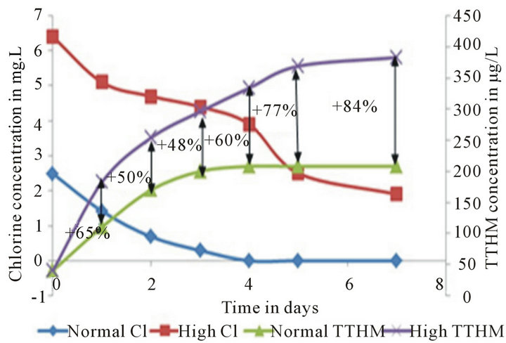
Figure 2. Normal run vs. high chlorine run chlorine residual and TTHM trends. The percent differences between the TTHM formation values are also noted.
support to kinetics analysis presented. Data collected satisfied ANOVA and paired t-test with 99% level of significance. Alpha value for 99% level of significance is 0.01.
According to the data presented above, it can be concluded that though High Chlorine Run can help maintain residuals over long time, the 84% increase in TTHM concentration is too high to ignore. Therefore, it’s in the utility’s interest to look for alternative ways to maintain chlorine residual for longer periods rather than adopting a High Chlorine approach.
3.2. Minimization of Wall Effects in High Chlorine Run
When kinetic coefficients of chlorine decay of the Normal Run are compared to the High Chlorine Run, in a Normal Run 34% of total chlorine decay can be attributed to bulk water reactions and the remaining 66% to wall reactions. Whereas, in a High Chlorine Run 82% of total chlorine decay can be attributed to bulk water reactions alone (Table 1).
With such drastic differences in the effects on wall and bulk reactions of chlorine decay between these two strategies, it can be concluded that High Chlorine conditions tend to increase the rate of bulk reactions, which minimizes wall effects on chlorine decay. This can be partially explained by the concept of collision theory, which states that presence of higher concentration of one reactant particles in a solution has a potential to change/ influence the reaction path, thereby affecting the concentration and type of products formed [23]. The High Chlorine scenario is one situation in which ignoring the wall reaction coefficient during calibration of physical or computer models can be justified. However, as with most distribution systems, the operation tends to be more chlorine-limited.
3.3. High Chlorine Run vs. Chlorine Booster Systems Run
This analysis is intended to statistically explain the merits and demerits of the two most common strategies used to maintain chlorine residual in long distribution systems or systems with higher chlorine demand. The primary purpose of both the High Chlorine run and the Chlorine Booster Systems Run is to help maintain required minimum chlorine residual in distribution systems. As explained earlier, the main difference between these two strategies is when and what amount of chlorine is added to the water. The data collected from the Loop shows that both strategies serve the purpose of residual maintenance over long periods of time very well while the difference is the concentration of regulated DBPs produced in the system (Figure 3).

Table 1. Kinetics data of all strategies: kinetics data of normal run and high chlorine run which reveals a less significant wall reaction rate coefficient observed for the High Chlorine situation.

Figure 3. High Chlorine Run vs. Chlorine Booster Run chlorine residual and TTHM trends. The percent differences between the TTHM formation and chlorine decay values are also noted.
According to the data presented above, it can be observed that High Chlorine Run does a really good job in maintaining chlorine residuals over long periods of time while Chlorine Booster Systems Run seem to do a better job than Normal Run (Figure 4), but not as good as High Chlorine Run in terms of maintaining residuals (Figure 3). An 86% decrease in chlorine residual can be observed in the Loop with Chlorine Booster System relative to High Chlorine system.
This can be attributed to the fact that High Chlorine Run started with about 156% higher chlorine concentration on Day 0. Though these two strategies started with the same amount of TTHM concentration on Day 0, on average the Chlorine Booster system produces 30% lower concentrations of TTHMs over a 4-day period.
This increase in TTHM concentration is solely due to an increase in amount of chlorine available in the system and can be explained as a product of an increase in the rate of reaction due a higher number of successful collisions.
Maintaining lower residual throughout the system helps in two ways: It ensures odor and taste quality of water and it decreases the amount of chlorine available in the system to form TTHMs. Therefore, based on the data analyzed as part of this research and prior knowledge of the odor and taste issues caused by higher amounts of chlorine in water, it can concluded that the Chlorine Booster System is a better solution for a utility with chlorine residual and TTHM issues. It helps maintain enough residual to be in compliance with minimum residual required in distribution systems regulation, taste and odor requirement, as well as decreases the potential to form high concentrations of TTHMs. It can be proven statistically with a 99% level of confidence that these two strategies produce different trends in chlorine decay and TTHM formation over time under constant wall conditions requiring utilities to be more careful when making the decision about using one strategy rather than the other. Data collected satisfied ANOVA and paired t-test with 99% level of significance. Alpha value for 99% level of significance is 0.01.
3.4. Chlorine-Limited Conditions in Distribution System
It is commonly accepted that most distribution systems are operated under chlorine limiting conditions [11,24- 28]. In order to understand the effect of chlorine limiting conditions in terms of water quality, data collected from the Loop under Normal Run and Chlorine Booster Run conditions are compared. Normal Run represents a system with chlorine-limited conditions while Chlorine Booster Run represents a system with continuous supply of chlorine at higher concentrations than Normal Run (Figure 4). Chlorine Booster Run, on average, maintained 3 times higher concentrations of residuals during 4-day run. The 11% increase in concentration of TTHM in the Booster run after boosting on Day 2 is solely due to increase in availability of extra chlorine residual in the system and the data shows about 104% increase of TTHM concentrations in Booster Run over the next 24 hours while the TTHM concentration seems to stabilize in Normal run. Stabilization of TTHM concentration in Normal Run is due to low to zero concentrations of chlorine available since everything else remained constant in the system. From this analysis it can be concluded that systems that are run under chlorine-limited conditions tend to provide better quality water in terms of TTHMs, odor, and taste when compared to systems that have higher chlorine residuals available such as Booster systems

Figure 4. Normal run vs. chlorine booster run chlorine residual and TTHM trends. The percent differences between the TTHM formation and chlorine decay values are also noted.
and High Chlorine systems. Therefore, maintaining lower residuals throughout distribution system can be considered as an optimal option for a utility both economically and in terms of water quality.
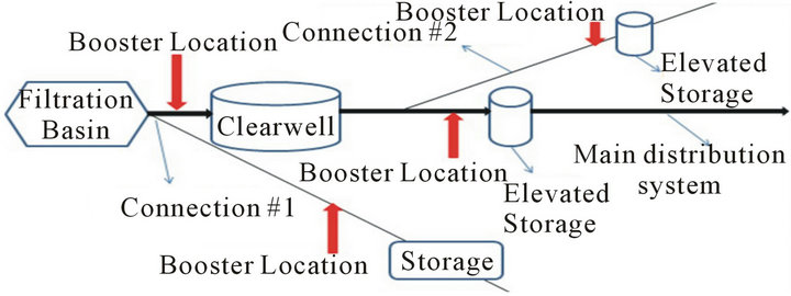
3.5. Location of Boosters
There are three ways utilities use chlorine boosters: 1) Within a single distribution system; 2) Before water leaves the treatment plant; 3) In consecutive systems. There are two options for chlorine booster placement in each of the above 3 usages (Figure 5).
Placement of chlorine boosters within a single distribution system with some kind of storage system in place requires the operators to make a decision whether to place the chlorine booster before or after the storage system (Figure 5).
In order to make this decision one has to know the effect of each option on water quality. Water quality in terms of TTHM formation is analyzed in this part of the research. The determination of an optimal location to place chlorine boosters can be done by answering the following question: “What happens to water quality when water entering the tank has concentrations of chlorine residual?” There are two ways to answer this question: 1) Run a scenario with low and high concentrations of chlorine entering the storage tank and study their effects on TTHM formation or 2) Determine the effect of higher chlorine concentration caused by a chlorine booster system on TTHMs formation relative to lower concentrations under normal conditions for the first 48 hours after boosting—assuming 48 hours would cover the travel time to storage tank and storage time in the tank (Figure 4).
An 11.5% increase in concentration of TTHM that was observed within 24 hours after boosting was solely due to
 (a)
(a)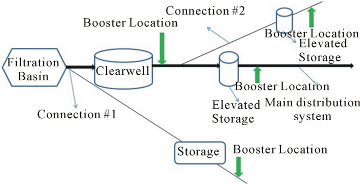 (b)
(b)
Figure 5. Chlorine booster system locations in distribution system in which (a) is considered poor locations and (b) is recommended locations.
the increase in availability of chlorine in the system and the data shows a 24% increase in TTHM concentrations by the end of the Booster Run. Therefore, in order to avoid such increase in TTHM concentrations during travel to storage tank and during storage in the tank, boosters need to be placed after the storage tank (Figure 5(b)).
This will reduce the contact time between additional chlorine and water as well as reduce the amount of chlorine used. In other words, water utilities need to add enough chlorine initially to get past the storage tank before using chlorine boosters; this will ensure lower concentration of chlorine in water entering the tank.
The concept of using chlorine boosters before the water enters the distribution system raises the question of need. Once the question about need is answered, the question about the placement of a chlorine booster system should be asked. There are two options for placement of the chlorine boosters with in the treatment plant (Figure 5): 1) Before or on top of the clearwell or 2) After the clearwell.
In order to make a decision about location of placement of chlorine boosters in this case, one needs to know what happens to water quality in terms of TTHM formation if water with high chlorine residauls enters the clearwell. There are two ways to know that: 1) Run a scenario in which water with high and low cocentrations of chlorine enters the clearwell and compare the TTHM concentrations to each other; 2) Run a set of Simulated Distribution System (SDS) tests with high and low concentrations of chlorine (Figure 6). High chlorine conditions tend to minimize the wall effects in the system (as explained earlier) therefore using SDS tests to analyze water chesmitry instead of actual clearwells is justified.
Addition of all the chlorine before filtration or placing a booster system before or on top of the clear well leads to a High Chlorine Run strategy inside the clear well which will minimize the wall effects. According to the bulk reactions data presented here, the TTHM concentration under high chlorine conditions is 78% higher than low chlorine conditions by the end of the 7-day run. Therefore, it can be concluded that usage of booster and placement of booster after the clear well is the optimal strategy for utilities (Figure 5(b)).
Based on the above analysis, it’s evident that placement of chlorine boosters after the storage tank/tower in consecutive systems is a better option (Figure 5). Placement of chlorine boosters plays a vital role in management of water quality in consecutive systems mainly because of the length of these systems and the fact that water would have travelled for days in primary distribution system before entering the secondary distribution network which usually leads to formation of TTHMs and loss of a considerable amount of residual.
4. Conclusion
High Chlorine run is least favorable option with approximately 64% and 30% higher production of TTHMs when compared to Normal and Chlorine Booster run, respectively. It is also determined that High Chlorine conditions minimize the wall effects with approximately 82% chlorine decay attributed to bulk reactions alone. Therefore, this is a situation where ignoring wall reaction coefficient for calibration of hydraulic/water quality models is justified. The location of Boosters should be after the storage systems to avoid extra contact time that can produce approximately 54% - 104% higher concentrations of TTHMs. This is proven to be true for boosters

Figure 6. SDS low chlorine (at 2.5 mg/L) vs. SDS High Chlorine (at 6 mg/L) chlorine residual and TTHM trends. The percent differences between the TTHM formation and chlorine decay values are also noted.
within a single distribution system and within a treatment plant. The water quality in distribution systems in terms of chlorine residual follows a HC > CB > NR trend and TTHM follows a NR > CB > HC operators need to realize that though a strategy like High Chlorine run can improve water quality in terms of one parameter, in this case chlorine, it can very much degrade in terms of others, which in this case happens to be TTHM. According to the data presented in this paper, Chlorine Booster system seems to be a better option to maintain water quality in long distribution systems, but compliance for stringent regulations such as Stage-II requires proper management of treatment process, booster locations, finding a right balance between system-specific conditions that may exist, and factors of variability of water chemistry in distribution systems.
5. Acknowledgements
Funding for this project was provided by National Institute of Hometown Security (NIHS). Analytical and technical support was provided by Missouri Water Resource Research Center (MWRRC) and Columbia Water Treatment Plant (CWTP).
REFERENCES
- R. Sadiq and M. J. Rodriguez, “Disinfection By-Products (DBPs) in Drinking Water and Predictive Models for Their Occurrence: A Review,” Science of the Total Environment, Vol. 321, No. 1, 2004, pp. 21-46. doi:10.1016/j.scitotenv.2003.05.001
- US Environmental Protection Agency, “National Primary Drinking Water Regulations: Disinfectants and Disinfection Byproducts,” Federal Register, Vol. 63, No. 241, 1998, pp. 69390-69476.
- B. Warton, A. Heitz, C. Joll and R. Kagi, “A New Method for Calculation of the Chlorine Demand in Natural and Treated Waters,” Water Research, Vol. 40, No. 15, 2006, pp. 2877-2884. doi:10.1016/j.watres.2006.05.020
- C. Adams, T. Timmons, T. Seitz, J. Lane and S. Levotch, “Trihalomethane and Haloacetic Acid Disinfection By- Products in Full-Scale Drinking Water Systems,” Journal of Environmental Engineering, Vol. 131, No. 4, 2005, pp. 526-534.
- J. Rook, “The Chlorination Reactions of Fulvic Acids in Natural Waters,” Environmental Science & Technology, Vol. 11, No. 5, 1977, pp. 478-482. doi:10.1021/es60128a014
- M. C. Besner, V. Gauthier, B. Barbeau and R. Millett, “Understanding Distribution System Water Quality,” Journal of the American Water Works Association, Vol. 93, No. 7, 2001, pp. 101-104.
- B. Carrico and P. C. Singer, “Impact of Booster Chlorination on Chlorine Decay and THM Production: Simulated Analysis,” Journal of Environmental Engineering, Vol. 135, No. 10, 2009, pp. 928-935.
- R. M. Clark and M. Sivaganesan, “Predicting Chlorine Residuals and Formation of TTHMs in Drinking Water,” Journal of Environmental Engineering, Vol. 124, No. 12, 1998, pp. 1203-1210. doi:10.1061/(ASCE)0733-9372(1998)124:12(1203)
- R. M. Clark, J. Q. Adams and B. W. Lykins, “DBP Control in Drinking Water; Cost and Performance,” Journal of Environmental Engineering, Vol. 120, No. 4, 1994, pp. 759-782. doi:10.1061/(ASCE)0733-9372(1994)120:4(759)
- R. M. Clark, “Chlorine Demand and TTHM Formation Kinetics: A Second Order Model,” Journal of Environmental Engineering, Vol. 124, No. 1, 1998, pp. 16-24.
- R. M. Clark, H. Pourmoghaddas, L. J. Wymer and R. C. Dressman, “Modeling the Kinetics of Chlorination ByProduct Formation: The Effects of Bromide,” Journal of Water Supply: Research and Technology-Aqua, Vol. 45, No. 3, 1996, pp. 112-119.
- N. B. Hallam, J. R. West, C. F. Forster, J. C. Powell and I. Spencer, “The Decay of Chlorine Associated with the Pipe Wall in Water Distribution Systems,” Water Research, Vol. 36, No. 14, 2002, pp. 3479-3488. doi:10.1016/S0043-1354(02)00056-8
- T. Haxton, R. Murray, W. Hart, K. Klise and C. Phillips, “Formulation of Chlorine and Decontamination Booster Station Optimization Problem,” World Environmental and Water Resources Congress (ACSE), Palm Springs, 22-26 May 2011, pp. 199-205.
- P. M. Jonkergouw, S. T. Khu, Z. S. Kapelan and D. A. Savic, “Water Quality Model Calibration under de Demands,” Journal of Water Resource Planning and Management, Vol. 134, No. 4, 2008, pp. 326-336.
- R. M. Clark and B. K. Boutin, “Controlling Disinfection By-Products and Microbial Contaminants in Drinking Water,” National Risk Management Research Laboratory, Office of Research and Development, Cincinnati, 2001.
- C. Li, J. Y. Yang, J. Yu, T. Zhang, X. Mao and W. Shao, “Second Order Chlorine Decay and Trihalomethanes Formation in Pilot Scale Water Distribution Systems,” Water Environment Research, Vol. 84, No. 8, 2012, pp. 656-661. doi:10.2175/106143012X13373550427390
- P. C. Singer, H. S. Weinberg, K. Brophy, L. Liang, M. Roberts, I. Grisstede, S. Krasner, H. Baribeau, H. Arora and I. Najm, “Relative Dominance of Haloacetic Acids and Trihalomethanes in Treated Drinking Water,” AWWA Research Foundation/American Water Works Association, Denver, 2002.
- D. L. Boccelli, M. E. Tryby, J. G. Uber and R. S. Summers, “A Reactive Species Model for Chlorine Decay and THM Formation under Rechlorination Conditions,” Water Research, Vol. 37, No. 11, 2003, pp. 2654-2666.
- S. R. Poleneni, “Analysis and Management of Disinfection By-Product Formation in Distribution Systems,” M.S. Thesis, University of Missouri, Missouri, 2013.
- APHA, AWWA and WEF, “Standard Methods for the Examination of Water and Wastewater,” 20th Edition, United Book Press, Baltimore, 1998.
- Hach, “Water Analysis Handbook,” 3rd Edition, Hach Company, Loveland, 1997.
- J. W. Munch, “EPA Method 524.2: Measurement of Purgeable Organic Compounds in Water by Capillary Column Gas Chromatography/Mass Spectrometry,” Office of Research and Development, Washington DC, 1995.
- C. G. Hill Jr., “Introduction to Chemical Engineering Kinetics and Reactor Design,” John Wiley & Sons, Inc., New Jersey, 1997.
- A. E. Germeles, “Forced Plumes and Mixing of Liquids in Tanks,” Journal of Fluid Mechanics, Vol. 71, No. 3, 1975, pp. 601-623. doi:10.1017/S0022112075002765
- W. M. Grayman and R. M. Clark, “Using Computer Models to Determine the Effect of Storage on Water Quality,” Journal of the American Water Works Association, Vol. 85, No. 7, 1993, pp. 67-77.
- M. S. Kennedy, S. Moegling, S. Sarikelli and K. Suravallop, “Assessing the Effects of Storage Tank Design,” Journal of the American Water Works Association (JAWWA), Vol. 85, No. 7, 1993, pp. 78-88.
- R. Mau, P. Boulos, R. Clark, W. Grayman, R. Tekippe and R. Trussel, “Explicit Mathematical Models of Distribution System Storage Water Quality,” Journal of Hydraulic Engineering ASCE, Vol. 121, No. 10, 1995, pp. 699-709.
- A. A. Zachár and A. A. Aszódi, “Numerical Analysis of Flow Distributors to Improve Temperature Stratification in Storage Tanks,” Numerical Heat Transfer: Part A— Applications, Vol. 51, No. 10, 2007, pp. 919-940. doi:10.1080/10407790601184405
NOTES
*Corresponding author.