Journal of Water Resource and Protection
Vol. 2 No. 11 (2010) , Article ID: 3188 , 12 pages DOI:10.4236/jwarp.2010.211114
Pool Effects on Longitudinal Dispersion in Streams and Rivers
Department of Civil and Environmental Engineering, Temple University, Philadelphia, USA
E-mail: boufadel@temple.edu
Received September 6, 2010; revised September 13, 2010; accepted October 11, 2010
Keywords: Pool effects, Solute transport, Longitudinal dispersion, Transient storage, Open channel
ABSTRACT
Surface storage (pools, pockets, and stagnant areas caused by woody debris, bars etc) is very important to solute transport in streams as it attenuates the peak of a spill but releases the solute back to the stream over a long time. The latter results in long exposure time of biota. Pools as fundamental stream morphology unit are commonly found in streams with mixed bed materials in pool-riffle or pool-step sequences. Fitting the transient storage model (TSM) to stream tracer test data may be problematic when pools present. A fully hydrodynamic 2-D, depth averaged advection-dispersion solute transport numerical simulation study on hypothetical stream with pool reveals that a pool can sharply enhance longitudinal spreading, cause a lag in the plume travel-time and radically increase solute residence time in the stream. These effects fade like a “wake” as the solute plume moves downstream of the pool. Further, these effects are strongly influenced by a dimensionless number derived from the 2-D transport equation − or
or , which outlines the relative transverse mixing intensity of a stream or river, where, of the stream reach concerned, W is the flow width, Q0 is the volumetric flow rate, q is the longitudinal flux density, and Dt is the transverse turbulent diffusion coefficient. The breakthrough curves (BTCs) downstream of a pool may be “heavy tailed” which cannot be modeled accurately by the TSM. The internal transport and mixing condition (including the secondary circulations) in a pool together with the pool’s dimension determine the pool’s storage effects especially when
  >> 1. Results also suggest that the falling limb of a BTC more accurately characterizes the pool's storage because the corresponding solute has more chance to sample the entire storage area.
1. Introduction
River and stream pollution is a serious global problem. It threatens the health and well being of humans, plants and animals.
Generally, pollutants are introduced into rivers and stream via point sources and non-point sources. The former includes either various accidental spills, or deliberate discharge of the effluent of wastewater treatment plant (WWTP) [1]. The latter refers to surface runoff which is recognized as a major source of pollutants to rivers and streams. The occurrence of pharmaceutically active chemicals (PACs) in the natural aquatic environment is recognized as an emerging issue due to the potential adverse effects these compounds pose to aquatic life and humans. The study of the fate of these human and veterinary pharmaceuticals (also called pharmaceuticals and personal care products (PPCPs)) has become an active investigation area [2,3], and the task as well as reducing the risk of various spills and mitigating the pollution cannot be done well without a good understanding of solute transport in streams.
Solute transport in streams or rivers refers to the spatial and temporal evolution of solute concentration in stream or river systems. A variety of processes determine the transport and fate of solutes within rivers and streams, e.g., the hydrological transport – physical process [4], geochemical processes, etc [5]. Aside from advection and dispersion that occur chiefly in the main channel, the hydrological transport is also affected by surface storage and hyporheic storage. In these storage zones, solute is temporarily trapped in either surface stagnant area (pools, pockets, etc.) or hyporheic zone (subsurface flow path surrounding the stream due to abrupt pressure change by meanders, pool-riffle series etc.). The detained solute is released after the solute concentration peak in the main channel passes. It is a dynamic process because of the continuous exchange between the active channel and the storage zones. These storage zones may strongly affect not only the hydrologic transport but also the total solute dynamics, e.g., the mass loading of solutes from terrestrial and atmospheric sources, the physical transport of solutes within the watershed, and the transformation of solutes due to geochemical and biogeochemical reactions in the hyporheic zone [6].
Solute transport modeling started from Taylor’s [7] classical and pioneering work. The landmark contribution of Fischer [8,9] and several researchers of his time significantly improve the simulation of longitudinal solute transport in open channel flow. Although the one dimensional advection-dispersion model (ADM) has been successfully used in many applications in streams of relatively uniform channels, it is not very successful in reproducing the transport in natural streams [4,10,11]. Many field studies as well as lab experiments reported long tailed breakthrough curves [8-10,12], meaning the processes were far from Fickian. Thus ignoring the positive skewness leads to overestimation of the peak concentration and underestimation of the residence time of contaminants in the stream system.
To tackle the non-Fickian process due to transient storage, numerous models have been developed. One of the widely used models is the “dead zone” model [10, 11,13], which is also known as transient storage model (TSM) [14]. TSM is a significant improvement over ADM, but it cannot be easily used as a predictive tool, more of an interpretive tool of solute transport. This is because a data set may simulate a particular stream reach very closely, and may be of little or no value for prediction outside or even in sub-reaches inside of that reach [15]. The mechanisms that govern longitudinal solute transport in some situations (e.g. the presence of pools) are not well understood.
Ge and Boufadel [15] conducted parameter estimation of the TSM by fitting the breakthrough curves (BTCs) of tracer test data sets from 3 consecutive sub-reaches in Indian Creek, Philadelphia, USA [16]. Although the model was able to closely fit the breakthrough curves at the end of the second and third subreaches, there were no parameter values that allow fitting to the breakthrough curve at the end of the first subreach, which was around 85 m downstream of the injection point. In particular there was not a parameter set that fits both the peak and the tail of the observed BTC. Ge and Boufadel [15] attributed the poorness of the fits to the presence of a large pool inside the reach. The pool had a cross-sectional area of 1.8 m2 in its mid-section, but the channels before and after the pool had cross-sectional areas of less than 0.5 m2. This abrupt enlargement of the channel caused incomplete mixing that violates the complete mixing assumption of TSM.
Pools are commonly found in streams with mixed bed materials in pool-riffle or pool-step sequences [17,18]. Thus, knowledge of the effects of a pool – large surface storage – is indispensable to understanding longitudinal solute transport in open channels. It is particularly important, for example, for the design of a constructed wetland to provide efficient supplemental treatment of the effluents of wastewater treatment plant (WWTP) in order to meet wildlife habitat goals [1]. However, not much attention has been paid to how a pool influences longitudinal solute transport in a stream.
We attempt to understand the role of a pool in a stream and its effects on solute transport by conducting numerical experiments using a two-dimensional (depth-averaged) model, MIKE21 (www.dhigroup.com) in a hypothetical, but realistic stream configuration. We consider four scenarios. The base scenario is of rectilinear stream with no pool within it. The three other scenarios are of streams that contain a pool of width 2 W, 4 W, or 7 W, where W is the width of the rectilinear stream.
The layout of the paper is as follows: First we present the governing equations for depth averaged water flow and solute transport in streams. These are the most rigorous equations for the two-dimensional problem. The equations are then rendered dimensionless using a unique non-dimensionalization approach, which would allow generalization of the results to a variety of stream systems. We then investigate the following: 1) pool effects on longitudinal solute transport; 2) the transport and mixing processes inside a pool.
2. Methods
MIKE 21 is a software package developed by DHI Water & Environment [19]. It is applied to simulation of hydraulics, water quality, tides, waves, and sediment transport in rivers, lakes, estuaries, bays, coastal areas and seas where stratification can be neglected. For our purpose, we will use MIKE21’s hydrodynamic (HD) and the advection-dispersion (AD) modules. The HD module solves the fully hydrodynamic 2-dimensional (i.e., depth averaged), free surface water flow equations. The AD module solves the two-dimensional equation for solute transport, which is the two-dimensional advection-dispersion equation.
2.1. The Hydrodynamic (HD) Model
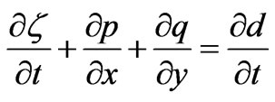
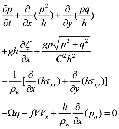
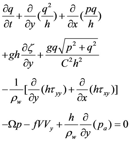
The two-dimensional equations of the hydrodynamic model in MIKE 21 [19] consist of the vertically integrated conservation of mass and momentum equations:
 (1)
(1)
 (2)
(2)
 (3)
(3)
Where,
 (x,y,t) surface elevation [m]
p (x,y,t), q(x,y,t) flux densities in x and y directions [m3s-1m-1]; p(x,y,t) = u(x,y,t) × h(x,y,t); q(x,y,t) = v(x,y,t) × h(x,y,t); u(x,y.t), v(x,y,t) are depthaveraged velocities in x and y–directions [ms-1]
d(x,y,t) time varying streambed elevation [m]
h(x,y,t) water depth [m], h =
g acceleration due to gravity [ms-2]
C(x,t) Chezy resistance [m1/2s-1], C =nh1/6, n is the manning number [m1/3s-1]
 w density of water [kg m-3]
x, y space coordinates[m]
t time[s]
 xx,
xx,  xy,
xy,  yy components of effective sheer stress [kg m-1s-2]
 (x,y,t) atmospheric pressure (kg/m/s2)
f(V) wind friction factor V,Vx,Vy(x,y,t) wind speed and components in xy- direction (m/s)
 Coriolis parameter, latitude dependent (s-1)
Equation (1) is the mass conservation equation. It states that the variation of the water mass in time (first term) is balanced by water flows in and out of a control volume along the stream (second term) and across the stream (third term). The right hand side term is zero in our experiments, because we are assuming that the streambed elevation d(x,y,t) does not vary with time. Equations (2) and (3) are the momentum equations. The first terms in Equation (2) and (3) relate to the temporal accelerations; the second and third terms are the spatial (or convective) acceleration terms; the fourth terms account for the gravity force; the fifth terms represent the force due to friction with the streambed; the next two terms represent internal friction within the fluid due to fluid viscosity; the last three terms – the Coriolis force, wind stress, and atmospheric pressure gradient – are beyond the scope of this study and will be omitted from this point on.
2.2. The Advection-Dispersion (AD) Model
The AD model simulates the transport of dissolved substances subject to advection and dispersion processes [19]. It solves the advection-dispersion equation:
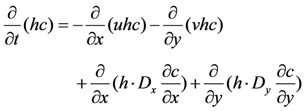 (4)
(4)
Wherec depth averaged solute concentration (arbitrary units)
h (x,y,t) water depth [m]
Dx, Dy dispersion coefficients in the x, y directions, respectively [m2s-1]
Equation (4) states that the variation of a conservative solute mass with time (left hand side) is equal to the solute flow in and out of the control volume due to convection (first two terms on the right hand side) and dispersion (the third and fourth terms on the right hand side) in the “2-D” space. The dispersion coefficients account for turbulent diffusion and the velocity shear that result from the variation of velocity in the vertical direction [20]. Dx, Dy are typically functions of space (x, y) but independent of time.
2.3. Description the Hypothetical Streams
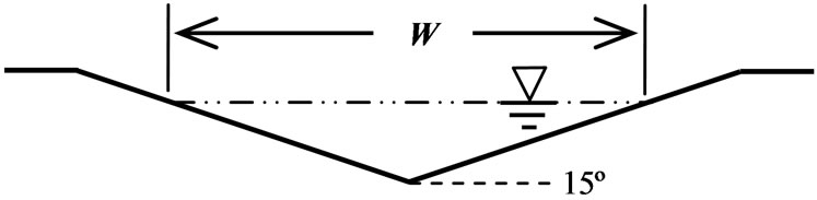
The main channel of each hypothetical stream was designed as a triangular cross-section and the pools were designed to have trapezoidal cross-sections with the same bank slope of 27% (Figure 1). There were four stream-pool configurations: (a) Stream with no pool, (b) Stream with a 2 W pool, (c) Stream with a 4 W pool, and (d) Stream with a 7 W pool. Longitudinally, the streams had a uniform slope of 0.1%. All the pools were located at the same location (with the outlet at x = 59.4 m). Table 1 contains additional stream details. Figure 2 is a 3-D realization of one of the hypothetical streams.
 (a)
(a) (b)
(b)
Figure 1. (a) Triangular main channel cross-section; (b) Trapezoidal pool cross-section. (Hypothetical streams simulated: 1W (i.e. no pool), 2 W, 4 W, and 7 W. Where W (= 3.8 m) was flow width of the main channel.)
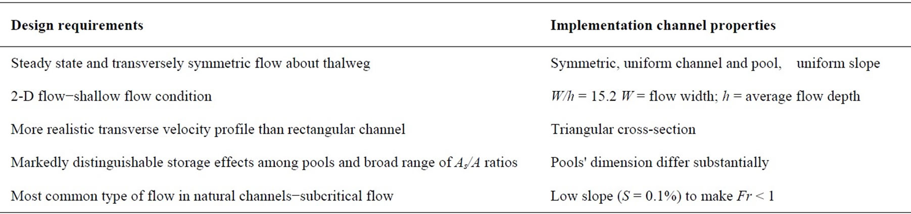
Table 1. Hypothetic stream property summary.
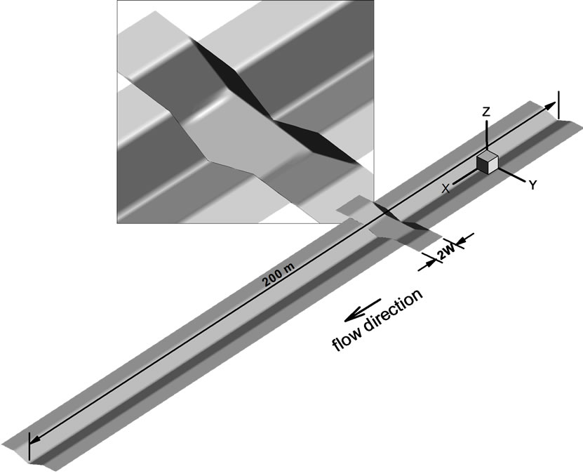
Figure 2. Hypothetical stream with a 2 W pool. (The lengths of pools were 2W for all. Where W (= 3.8 m) was flow width of the main channel. (Size Factor X: Y: Z = 2.69:1.00:6.19))
The width W was taken to be 3.8 m; the cross-sectional area of the flow was 0.938 m2, however, the dimensionless formulation that we developed (See Appendix) ensures that our results apply to a wide range of natural conditions. Simulations were presented as function of the dimensionless group :
:
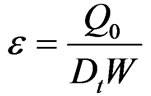 (5)
(5)
where Q0 is the discharge, Dt is the transverse dispersion coefficient, and Wis the flow width. Thus,  represents the ratio of longitudinal convective transport to transverse dispersive transport. It has, thus, the significance of a physical Peclet number. Large
  (>> 1) corresponds to high longitudinal mass transport by convection or weak transverse dispersion.
We selected four values of  (0.27; 1.08; 3.00; and 5.41) for each geometric configuration. The range of
  is observed in natural streams/rivers. For example, Bear Creek, Colorado (
 = 3.88); Nooksack River, Wash. (
 = 4.17 and 3.77); Copper Creek, Va. (
 = 5, 2.15 and 4.17); Powell River, Tenn. (
 = 4.01); Conococheague Creek, Md. (
 = 3.08).
2.4. Mike21 HD AD Model Set Up
A horizontal grid of 0.2 m × 0.2 m was used, which resulted in 19,000; 19,361; 20,083; and 21,166 blocks for the pool-stream configurations of no-pool, 2 W pool, 4 W pool, and 7W pool, respectively. Note that the length of the pools was always 2 W. A FORTRAN code was used to generate the digitized bathymetries.
In each simulation, the upstream boundary condition was set as a distributed flux, see Figure 3; the downstream boundary condition was set as given water level equals to -0.2537 m. Small time steps were used to make the maximum Courant number, Cr, less than 1 [19]. The model was run until hydraulic steady state prior to injection of the tracer. The hydrodynamics in the pools at steady state is reported in Figure 4.
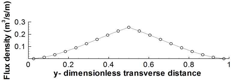
Figure 3. Upstream flux density boundary condition.
 (a)
(a)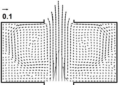 (b)
(b)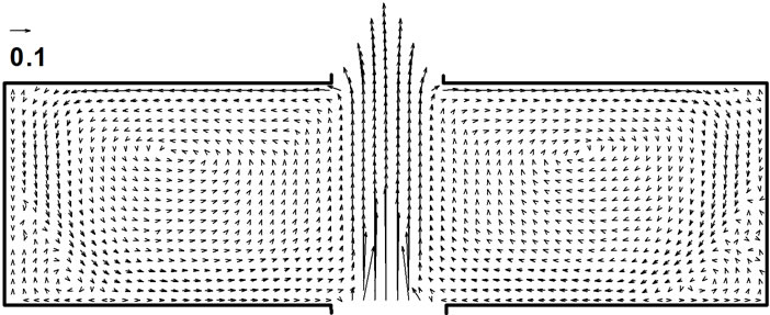 (c)
(c)
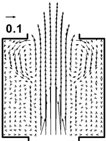
Figure 4. Velocity distributions (vector plots) of the pool areas. (a) 2 W pool; (b) 4 W pool; (c) 7 W pool.
The injection location was at the upstream boundary. The dispersion coefficient was considered as isotropic, i.e. 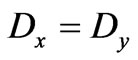 = D (a constant). In each simulation, a mass flux boundary condition of a conservative tracer was applied uniformly across the stream. The mass flux was equal to 164.3 mg/s; the injection lasted 16 seconds. The concentration at the source was 400 mg/m3.
Because of the restriction of the numerical platform we used - Mike 21 version 2005 and 2003, we were not able to simulate situations with vary bed resistance and turbulent diffusion coefficients especially in the pool. Although a more detailed two- (or perhaps three-) dimensional analysis may be needed to get a complete delineation of pool effects, the results of this study provide an elementary but very important understanding of pool effects on longitudinal spreading in a stream or river. Simulations in this study were limited to the pulse-like injection only. Increase injection time will raise a pool’s exposure to solute cloud, and some of the reported results herein will thus be changed in form. The focus of this study was the mechanisms that govern how a pool influences longitudinal solute transport, but not quantifying a pool’s storage, and so the injection adopted herein – a pulse-like input – is reasonable.
3. Results and Discussion
Two-dimensional breakthrough curves were obtained at cross-sections 2 W upstream of the pool, and 2 W, 10 W, 20 W and 30 W downstream of the pool. They were also obtained at the following transverse distances from the center axis: 0.0 W (stream center), 0.1 W, 0.2 W, 0.32 W, and 0.42 W, where W is the channel flow width. Note that the results were symmetric with respect to the channel thalweg.
The 2-D BTCs were converted into 1-D BTCs by averaging arithmetically across the channel because the primary purpose of this paper was to study the longitudinal dispersion. The averaged BTCs were reported in groups according to the dimensionless number .
.
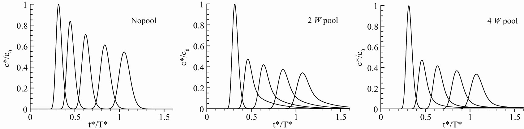
Figures 5 through 8 report the BTCs for all cases. As there is too much information in the figures to zoom in while showing all the breakthrough curves, we focus on the following properties: The peak concentration, the time of the peak, the fall-off of the tail, and the mass stored in the pools.
3.1. The Attenuation of the Peak Concentration
The decrease of the peak for the no-pool case was gradual until the end of the stream (at x = 30). However, a sudden decrease of the peak concentration was noted immediately after the pools for all  values (Figure 9).
 (a)
(a)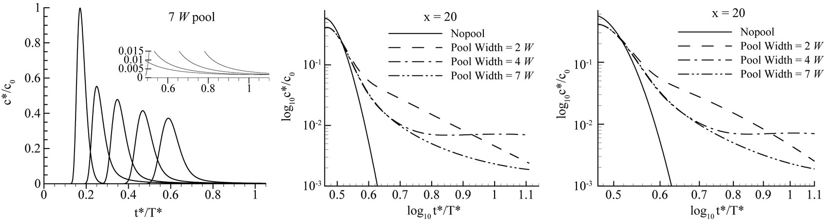 (b)
(b)
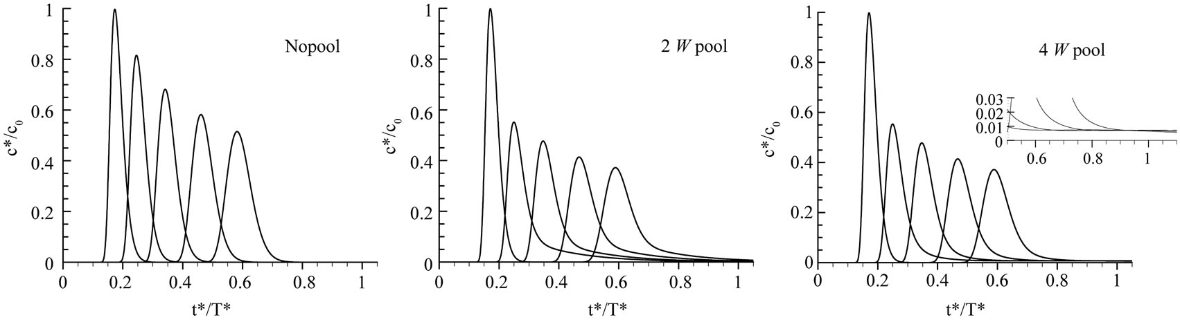
Figure 5. Simulation results, ε = 5.41. (a) – (d) BTCs at 5 locations: from left, 2 W upstream of the pool, 2 W, 10 W, 20 W, and 30 W downstream of the 1 W, 2 W, 4 W, 7 W pool, respectively; (e) semi-log plot of the falling limbs; (f) log-log plot of the falling limbs, where W = 3.8m. c* is the tracer concentration [M/L-3]; c0 is the tracer concentration at 2 W upstream of the pool; t* is the time after injection [T]; T* = W*2/Dt, where W* is a characteristic length = W, Dt is the transverse dispersion coefficient.
 (a)
(a)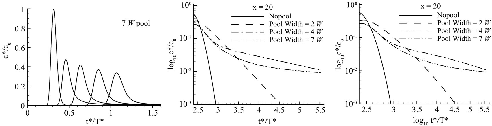 (b)
(b)
Figure 6. Simulation results, ε = 3.00. (a) – (d) BTCs at 5 locations (from left, 2 W upstream of the pool, 2 W, 10 W, 20 W, and 30 W downstream of the 1 W, 2 W, 4 W, 7 W pool, respectively); (e) semi-log plot of the falling limbs; (f) log-log plot of the falling limbs.
 (a)
(a)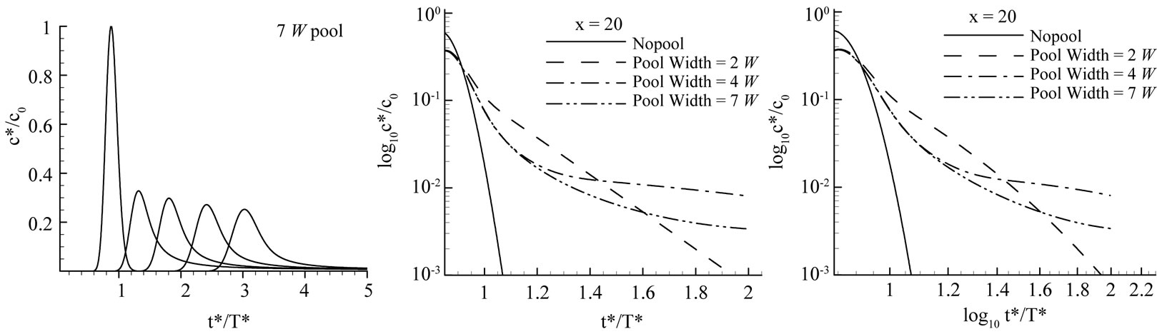 (b)
(b)
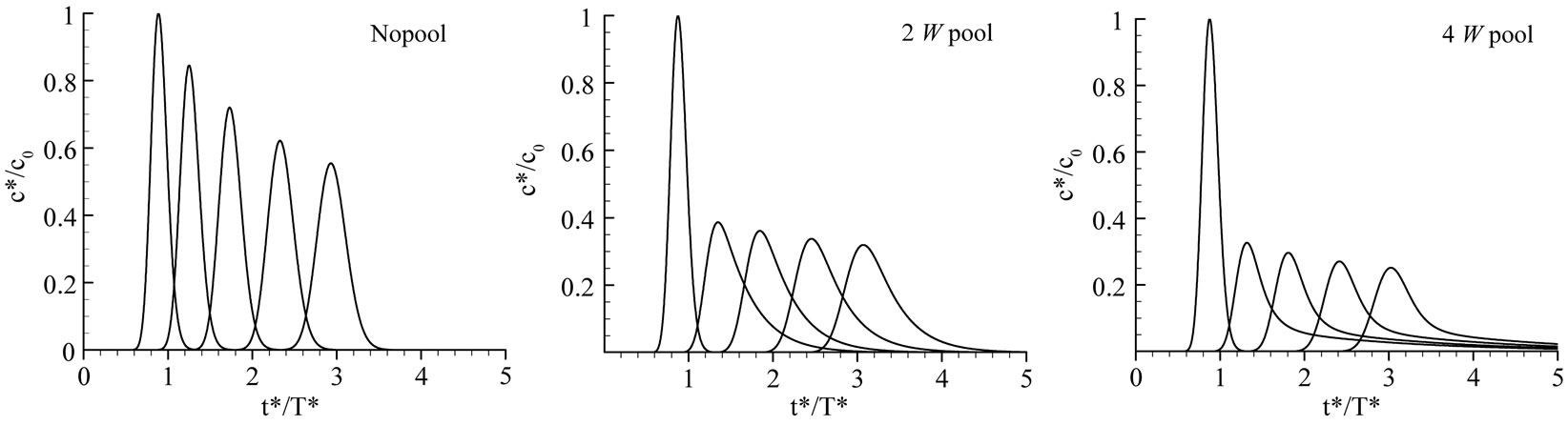
Figure 7. Simulation results, ε = 1.08. (a) – (d) BTCs at 5 locations (from left, 2 W upstream of the pool, 2 W, 10 W, 20 W, and 30 W downstream of the 1 W, 2 W, 4 W, 7 W pool, respectively); (e) semi-log plot of the falling limbs; (f) log-log plot of the falling limbs.
 (a)
(a)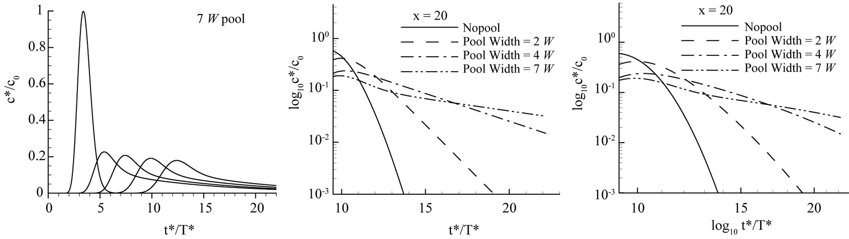 (b)
(b)
Figure 8. Simulation results. ε = 0.27. (a) – (d) BTCs at 5 locations (from left, 2 W upstream of the pool, 2 W, 10 W, 20 W, and 30 W downstream of the 1 W, 2 W, 4 W, 7 W pool, respectively); (e) semi-log plot of the falling limbs; (f) log-log plot of the falling limbs.
For  larger than 3.00, the peak values were the same regardless of the size of the pools. This is an important finding indicating that complete mixing of the solute in the pool did not take place (otherwise the 7 W pool would result in smaller peak), which is a common assumption in stream studies.
The effect of pool size became important at  = 1.08 where the peaks of the 4 W and 7 W were less than those of the 2 W pool by about 15%. The case of
  = 1.08 is particularly interesting, as the peak value at the exit of the 2 W pool was larger than that obtained from other
  values (namely
  = 3.00, 5.41). An explanation for this is related to dispersion in the axial direction. As we assumed that the two-dimensional transverse dispersion coefficient Dy is equal to the two-dimensional longitudinal dispersion coefficient Dx, a decrease in
  results in a decrease in both Dy and Dx. When
  = 5.41, this means that transport by convection (in the longitudinal direction) is 5.41 times of the transport by dispersion in the longitudinal direction. When
  reaches the value of 1.08, this implies that transport by convection is comparable to that of dispersion in the longitudinal direction. This caused the rapid fill up of the 2 W pool with a high concentration in both the transverse and longitudinal direction, and resulted in a “spill” of high peak concentration at the exit in comparison with other
  values. For the 4 W and 7 W cases, the transverse dispersion was not able to fill the pools in the transverse direction before the plume emerged out of the pool, as the length of the pools was 2 W. One might argue that the small values of
  are theoretical. However, this has to be considered in the context of parameterization and scale. For example, if the pool’s bathymetry causes the water to move transversely (say to the presence of a gravel bar, a boulder, or a tree in the middle of the pool) then the “effective” transverse dispersion would be large. Of course, if one elects to model the details of water flow within the pool (i.e., transverse convection) then such an effective transverse dispersion disappears at the scale of the water pathways. But when treating the pool as a hydraulic unit, transverse convection would need to be treated as an effective transverse dispersion.
An important observation in Figure 9 is that the reduction of the peak concentration with downstream distance after the pools was mild in comparison with the rectilinear stream (i.e., no pool). This is due to the slow release of solutes from the pool which sustain the solute in the stream for long durations. Accounting for the presence of the pool is of extreme importance when dealing with actual spills (especially of hazardous material); if one were to measure the concentration at x = 2 W in a stream that has a pool, and if one were not aware of the presence of a pool, then one would expect a relatively large decrease in peak concentration going downstream, which would underestimate the impact on the environment.
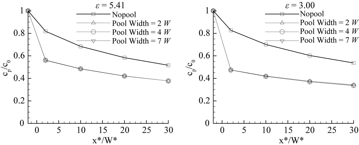
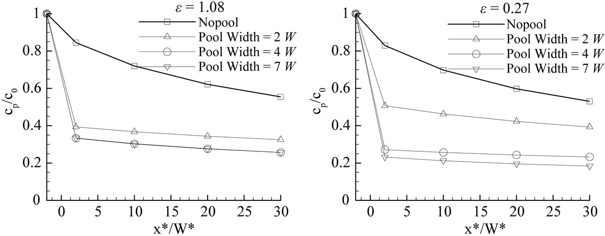
Figure 9. Variation of the dimensionless peak concentration with dimensionless downstream distance, where cp is the peak concentration [ML-3]; c0 is the concentration at 2 W upstream of a pool [ML-3]; x* is the distance from a pool [L]; W* = W [L].
3.2. Lag of Concentration Peak
The pools delayed the concentration peak travel-time with respect to the no-pool case. As a matter of fact, the pools delayed the whole solute plumes. The delay was computed as:
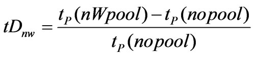 (6)
(6)
As shown in Figure 10, the delays increased sharply with decreasing . At 2 W downstream of the pools and
  = 0.27, the 2 W pool, 4 W pool, and 7 W pool caused delays of 13.6%, 16.1%, and 10.6% of the no-pool reference travel-time. Notice that the 7 W pool caused less delay than the 2 W pool in this case. This inconsistency has something to do with the internal transport and mixing which is strongly affected by the secondary circulations in a pool. Table 2 and Figure 4(a) (b) (c) show that the 2 W pool had the strongest secondary circulation and irregular flow pattern, which enhanced both transverse transport across the pool-channel interface and the transport and mixing inside the pool. The 7 W pool had the weakest current and well organized (smooth) flow pattern, which does not engender mixing; the 4 W pool’s behavior was intermediate. The difference of the secondary circulations together with pool size come into play in determining pool effects when relative transversemixing intensity become strong enough (characterized by small
  e.g.
e.g.  = 0.27). This strong relative transversemixing ensures long enough effective contact time–the dimensionless time–to make the solute cloud sample the entire pool (deadzone).
Then why the 2 W pool caused more peak travel-time delay than the 7 W pool? It is because the stronger internal transport and mixing due to stronger secondary circulation made the 2 W pool “absorb” the cloud more efficiently than the 7 W pool as the “same” solute cloud passing by. However, the zero concentration gradient across the storage-active channel interface, or conditionally “saturated” state of storage came earlier due to both the stronger internal transport and mixing and the much smaller storage capacity. Starting from the saturated state when the detained solute reached maximum, the 2 W pool began to “exude” solute from it; on the other hand, although the 7 W pool “absorbed” the solute plume not as efficiently, it maintained the “negative concentration gradient” which drove the solute into the pool for much longer time due to its much larger size and ended up with more solute absorbed in it than in the 2 W pool. The 4 W pool had stronger secondary circulation than the 7 W pool and much larger size than the 2 W pool, and hence held back the breakthrough most. Therefore, secondary circulation is another key factor influencing pool effects on longitudinal transport.
Figure 10. Delay of dimensionless peak travel-time increased with decreasing e.
Table 2. Speed distribution in pool areas.
The delay of the peak travel-time did not demonstrate signs of diminishing in our simulations. The travel-times increased linearly with distance.
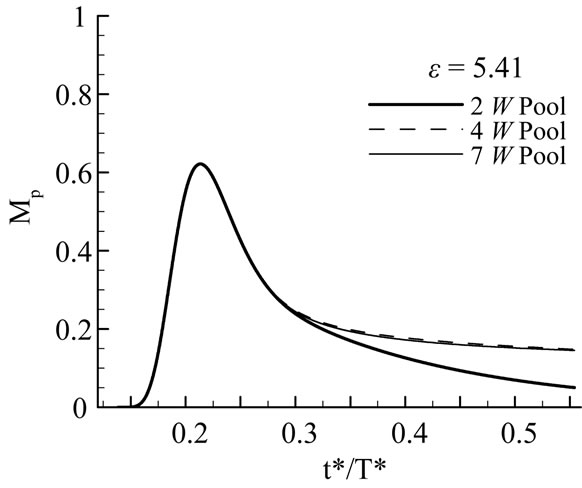
Figure 11 reports the variation of mass stored in the pool, Mp, as a function of time for various pool widths and various epsilon values. As seen in Figure 11(a), (b), maximum detained solute in the pools was affected by e mainly, and pool size did not affect the entire accumulating and partial of the depleting processes; it is interesting that the turning point was around  = 1.0 under these experiment conditions, and the maximum quantity of the accumulated solute was about 80% of the total injected in the 2 W pool ( Figure 11 (c)); Pool size came into play regarding the accumulating and depleting processes (Figure 11(d)). Notice that the pool area (the main channel area (2 W × W) subtracted from the total “gross” pool area (2 W × n W, n = 2, 4, 7)) which we computed the accumulated solute mass is different from the deadzone area (a cross-sectional area) defined by the TSM1, but they seemed to be closely correlated.
3.3. The Skewness of the BTCs
The pools made the BTCs skew as well. A comparison of the BTCs in Figure 5(b), Figure 6(b), Figure 7(b), and Figure 8(b) indicates that the skewness or tails would vanish (i.e., become Gaussian) with decreasing . Nevertheless, for a given
  as seen in Figure 8, the tracer cloud would eventually become Gaussian which is clearly demonstrated in Table 3. Notice that the BTC will not be strictly Gaussian due to longitudinal dispersion occurs during the time taken for tracer cloud to pass a fixed sampling site [20].
The skewness g(x) is calculated as
 (7)
(7)
Where,  is the total mass injected;
  is the mean travel-time of the solute cloud; c(x,t) is the solute concentration in stream, x is the distance from a reference location and we
 (a)
(a)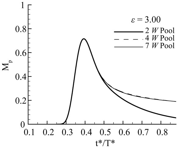 (b)
(b)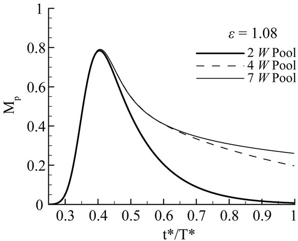 (c)
(c)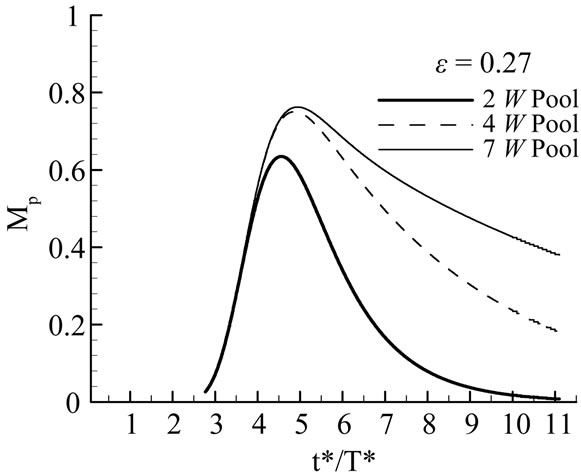 (d)
(d)
Figure 11. Solute accumulation in the pool areas.
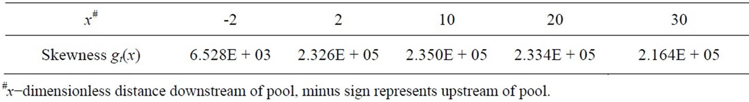
Table 3. Skewness change of 2 W-pool stream (pool was located at x = 0).
set the origin of x coordinate at the outlet of the pool, t is the time after a pulse injection. In Figure 12, breakthrough curve A is approximately symmetric about μt1 because of no storage effects, so, 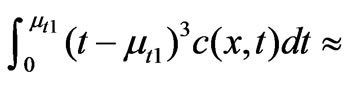 -
-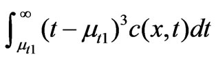 , and
, and ; Curve B skews because of storage (e.g. a pool), so,
  >
>  due to the radical increase of
 and the gradual decrease of
 , so,
, so,  > 0. The more skewed the BTC (the longer the tail2), the greater the
 .
.
A pool keeps stretching a plume during its “passage”. If Lmax is the extent from the pool outlet to the location of the plume front immediately after the plume “passes” the pool (i.e.,  is sufficiently close to zero to make the product
 ·
· negligible), then Lmax represents the plume’s maximum “stretch” caused by the pool, and
  reaches its maximum at x = Lmax. Within 0 – Lmax,
  increases in the flow direction; beyond x = Lmax,
  decreases, and the plume starts to evolve to Gaussian [9]. Table 3 presents the quantitative analysis result that clearly reveals the pattern of the skewness change. The skewness grew and then decreased instead of increasing or decreasing monotonically. We call this change pattern, together with the other two pool’s effects, “wake” effect just like the downstream disturbed flow caused by the relative motion between a solid body and a fluid. Obviously, Lmax (2 W pool) << Lmax (4 W pool)
Of the three-fold “wake” effect: concentration peak attenuation (longitudinal spreading acceleration), tailed BTC and delay of peak travel-time, peak travel-time delay is the only non-diminishing aspect. However, the cloud will become so spread out after sufficiently long distance downstream that the lag simply becomes trivial. Thus, in this respect, the “wake” fades, too.
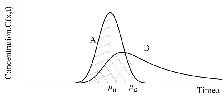
Figure 12. Skewness  (third-order temporal moment).
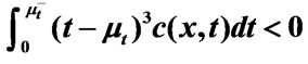 ;
; .
. ,
, : mean travel times of the plumes. Curve A, symmetric (no storage),
  = 0; Curve B, skewed (due to storage),
  > 0.
> 0.
For larger  (Figure 5 and 6), the rising limbs did not uniquely identify the pools, while the falling limbs especially the “late-time” behaviors discriminated from each other: virtually Gaussian for the no pool case; exponential for the 2 W pool; the 4 W pool and 7 W pool show very slow decaying tails suggesting very long residence time for some solute detained in these pools (see Figure 5(e)(f) and Figure 6(e)(f)). With decreasing
 , the rising limbs more and more discriminated different pools. There seemed to be a turning point around
  = 1.08 Figure 7). The differences of the BTCs among the 3 pools became evident after the turning point. The falling limbs especially the late-time transport behaviors discriminated noticeably: virtually Gaussian for the no pool case; exponential for the 2 W pool and the 4 W pool (see Figure 7(e)); the 7 W pool showed very slow decaying tails still (Figure 7(f)). For very small
  (Figure 8 (e)(f)), the BTCs of different pools distinguished from each other significantly: while the BTC of the 2 W-pool stream maintaining exponential but approaching to Gaussian, the late-time behavior of the 4 W and the7 W pool inclined to exponential, and more and more discriminating rising limbs emerged. Although the simulation time of our results was not long enough to display the well established late-time behavior, we conjecture the BTC tails of surface storage, from a spectrum of a side pocket to a large artificial swamp, may vary from exponential to those match the typical hyporheic storages (e.g., lognormal, power-law). Solute corresponding to the rising limb especially the earlier time of the BTC may have less chance to sample the entire pool (deadzone) area than that corresponding to the falling limb of the BTC. Fitting the whole BTC to parameterize the TSM therefore leads to the problem addressed by Ge and Boufadel [15].
4. Conclusions
A pool (large surface storage) can significantly enhance longitudinal dispersion in a stream or river. We conjecture the BTC tails of surface storage, from a spectrum of a side pocket to a large artificial swamp, may vary from exponential to those match the typical hyporheic storages. Acceleration of spreading, delay of travel-time, and long tail of the BTC manifest a pool’s effects on longitudinal solute transport. These effects are strongly influenced by the dimensionless number . However, the spreading enhancement is limited in a certain extent because, as the solute cloud propagates downstream, a pool’s aforementioned effects fade in one way or another like a “wake” (e.g. the BTC has finite third order moment – skewness). The secondary circulation induced transport and mixing is another important factor determining the pool’s storage effects. It suggests that when
  >> 1 (that is the case for most natural streams/rivers), the falling limb bears more information about a pool (storage) than the rising limb.
5. Acknowledgements
Our sincere thanks to all those who have helped us in this work, directly or indirectly. Especially the authors would like to thank Dr. Robert J. Ryan for his help with improving the writing of the earlier version of this paper. This work was supported in part by a grant from the USDA PENR-2003-01280. Wei Zhang was partially supported by a Temple University Scholarship. No official endorsement should be inferred from the funding sources.
REFERENCES
- S. H. Keefe, L. B. Barber, R. L. Runkel, J. N. Ryan, D. M. McKnight, and R. D. Wass, “Conservative and reactive solute transport in constructed wetlands,” Water Resources Research, vol. 40, W01201, 2004, pp. 12.
- J. G. M. Derksen, G. B. J. Rijs and R. H. Jongbloed, “Diffuse Pollution of Surface Water by Pharmaceutical Products,” Water Science and Technology, vol. 49, no. 3, pp. 213-221, 2004.
- M. Velicu and R. Suri, “Presence of steroid hormones and antibiotics in surface water of agricultural, suburban and mixed-use areas”, Environ Monit Assess, vol. 154, 2009, pp. 349-359.
- H. B. Fisher, E J. List, R. C.Y. Koh, J. Imberger and N.H. Brooks, “Mixing in inland and coastal waters,” Academic Press, 1979.
- J. R. Webster and T. P. Ehrman, “Solute Dynamics,” In: F. R. Hauer and G. A. Lamberti, ed., Methods in Stream Ecology, Academic Press, Inc., San Diego, Calif., 1996, pp. 145 -160.
- R. Runkel, D. M. McKnight and H. Rajaram, “Modeling hyporheic zone processes”, Advance Water Resources, vol. 26, no. 9, 2003, pp. 901-905.
- G.I. Taylor, “The dispersion of matter in turbulent flow through a pipe,” In: Proceedings of the Royal Society London Series A, vol. 123, 1954, pp. 446-468.
- H.B. Fischer, “The Mechanics of Dispersion in Natural Streams,” Journal Hydraulics Division Proceedings, ASCE, vol. 93, no. 6, 1967, pp.187-216.
- H.B. Fischer, “Dispersion Predictions in Natural Streams,” Journal Sanitary Engineering Division, ASCE, vol. 94, no. SA5, 1968, pp. 927-943.
- E. L Thackston, and K. B Schnelle, “Predicting effects of dead zones on stream mixing”. Journal of the Sanitary Engineering Division. Proceeding of The American Society of Civil Engineering, vol. 96, no. 2, 1970, pp. 319- 331.
- K. E. Bencala and R. A. Walters, “Simulation of solute transport in a mountain pool and riffle stream: a transient storage model,” Water Resources Research, vol. 19, no. 3, 1983, pp. 718-724.
- C. F. Nordin and B. M. Troutman, 1980. “Longitudinal dispersion in rivers: the persistence of skewness in observed data,” Water Resources Research, vol. 16, no. 1, 1980, pp.123-128.
- E. M. Valentine, and I. R. Wood, “Longitudinal dispersion with dead zones”. Journal of the Hydraulics Division, vol.103, no. HY9, 1977, pp. 975-991.
- R. L. Runkel, “One-dimensional transport with inflow and storage (OTIS): a solute transport model for streams and rivers (WRIR 98-4018),” US Geological Survey, Denver, CO 73 pp. 1998.
- Y.Ge and M. Boufadel, “Solute transport in multiple-reach experiments: Evaluation of parameters and reliability of prediction,” Journal of Hydrology, vol. 323, no. 1-4, May 2006, pp. 106-119.
- M. Gabriel, “The role of geomorphology in the transport of conservative solutes in streams. M.S. thesis, Temple University, Philadelphia, 2001.
- P. A. Carling and H.G. Orr, “Morphology of riffle-pool sequences in the river severn,” England. Earth Surface Processes and Landforms, vol. 25, no. 4, 2000, pp. 369- 384.
- A.Chin, “The periodic nature of step-pool mountain streams,” American Journal of Science, vol. 302, February 2002. pp. 144-167.
- DHI Water and Environment, 2003. MIKE 21- Coastal Hydraulic and Oceanography(Hydrodynamic Module: Scientific Documentation; Advection-Dispersion Module: Scientific Documentation).
- J. C. Rutherford, “River mixing,” John Wiley and Sons, New York, 1994.