Journal of Biomedical Science and Engineering
Vol.7 No.9(2014), Article ID:47905,13 pages
DOI:10.4236/jbise.2014.79066
Comparison between Different ESI Methods on Refractory Epilepsy Patients Shows a High Sensitivity for Bayesian Model Averaging
Danilo Maziero¹, Agustin Lage Castellanos², Carlos Ernesto Garrido Salmon¹, Tonicarlo Rodrigues Velasco³
1Department of Physics, FFLCRP, University of São Paulo, Ribeirão Preto, Brazil
2Cuba Neuroscience Center, Havana, Cuba
3Epilepsy Surgery Center, Department of Neuroscience, Faculty of Medicine, University of São Paulo, Ribeirão Preto, Brazil
Email: danibeen@hotmail.com
Copyright © 2014 by authors and Scientific Research Publishing Inc.
This work is licensed under the Creative Commons Attribution International License (CC BY).
http://creativecommons.org/licenses/by/4.0/


Received 6 May 2014; revised 20 June 2014; accepted 1 July 2014
ABSTRACT
Electrical Source Imaging (ESI) is a non-invasive technique of reconstructing brain activities using EEG data. This technique has been applied to evaluate epilepsy patients being evaluated for epilepsy surgery, showing encouraging results for mapping interictal epileptiform discharges (IED). However, ESI is underused in planning epilepsy surgery. This is basically due to the wide availability of methods for solving the electromagnetism inverse problem (e-IP) associated to few studies using EEG setups similar to those most commonly used in clinical setting. In this study, we applied six different methods of solving the e-IP based on IEDs of 20 focal epilepsy patients that presented abnormalities in their MRI. We compared the ESI maps obtained by each method with the location of the abnormality, calculating the Euclidian distances from the center of the lesion to the closest border of the method solution (CL-BM) and also to the solution’s maxima (CL-MM). We also applied a score system in order to allow us to evaluate the sensitivity of each method for temporal and extra temporal patients. In our patients, the Bayesian Model Averaging method had a sensitivity of 86% and the shortest CL-MM. This method also had more restricted solutions that were more representative of epileptogenic activities than those obtained by the other methods.
Keywords:EEG, Epilepsy, Electrical Source Imaging, Bayesian Model Averaging

1. Introduction
Epilepsy surgery may be a plausible option for drug resistant patients. However, the surgical planning has to be a very cautious procedure, based on information obtained by the agreement among different techniques, such as the ictal and interictal electroencephalogram (EEG), magnetic resonance imaging (MRI), positron emission tomography (PET), single photon emission computerized tomography (SPECT) and magnetoencephalogram (MEG). Unfortunately, in some patients the information available by these non-invasive techniques is not enough to identify the epileptogenic area, the brain area needed to be resected in a surgery in order to make the patient seizure-free. In such patients further investigation is needed, which is generally done by invasive methods, such as intracranial or foramen ovale electrodes, which carry considerable morbidity and cost.
A non-invasive method based on the application of the electromagnetism inverse problem (e-IP) [1] on EEG data is the Electrical Source Imaging (ESI). ESI, briefly, is capable to reconstruct a three dimensional source within the brain that generated the electrical potential differences measured by electrodes positioned on the scalp. The e-IP is an ill-posed problem and needs to be constrained to be solved. There are many methods used to constrain the e-IP obtaining the ESI, and they are based on different mathematical and physiological assumptions, for example the method Equivalent Dipole (ED) [2] , which groups the solution as an electrical dipole assumed to occupy a single point within the brain. Other methods as Minimum Norm (MN) [3] , Low Resolution Electromagnetic Tomography (LORETA) [4] , Local Auto-Regressive (LAURA) [5] , Classical LORETA Analysis Recursively Applied (CLARA) [6] and Bayesian Model Averaging (BMA) [7] consider the source responsible for generating the electrical currents with a finite extension.
The implementation of ESI methods and their capabilities to reconstruct the electrical sources detected by the scalp EEG has been reported for many studies, in simulated [6] [8] [9] and in real EEG data [6] [9] [10] . Some of these methods have been applied on experimental data [9] , others as the BMA has arisen as a potential tool, basically in evaluations over simulated and real task related data [6] , but it has not been applied so intensively on clinical EEG data such as on EEG data of epilepsy patients. Briefly BMA is a statistical method based on the possibility of incorporating a priori anatomical and/or functional information for estimating the sources [7] . Therefore its estimations are capable to relate the source to the patient a priori known anatomical and functional information.
In epilepsy the ESI application is generally based on the interictal epileptic form discharges (IEDs) detected by the scalp EEG. There are many studies reporting good results about the use of ESI to localize the epileptogenic electrical activity [10] -[16] , but there is not many studies comparing different methods of solving the inverse problem of EEG data acquired in the clinical routine of epilepsy. Although the ESI has been proven to be a helpful method in localizing the epileptogenic zone, it has been underused in the clinical routine related to epilepsy.
The underuse of ESI in the clinical routine of epilepsy is partially explained for three reasons: 1) There are many methods available for solving the inverse problem. 2) The number of electrodes usually applied in clinical routine to acquire the EEG data usually ranges from 16 to 60 electrodes, which is fewer than the number used in the studies for proving the ESI applicability (>128 electrodes). 3) The ESI accuracy reported in literature shows different values for studies including epilepsies located in different lobes. These studies generally group the patients as temporal lobe patients and extra temporal patients, and there is no consensus about the group that can have the IED-related activity more accurately mapped. There is an argument that there is a lower accuracy for mapping the IEDs-related activities intemporal patients, which relates to the inaccuracy of detecting discharges originated in deep brain structures by scalp-EEG.
In this study, we applied six different methods of solving the inverse problem on EEG data of 20 patients with focal epilepsy. Then, we compare the solution obtained by each method with the location of an abnormality in the patient’s MRI. We calculated the distance from the lesion to the solution closest border and also to the maximum of the solution. Finally, we grouped our results based on the likely epileptogenic region location in order to compare the accuracy of each method for mapping epileptogenic zones originated in temporal and extra-temporal lobes.
2. Methods
2.1. Patients
Patients were selected from our clinical database by the following inclusion criteria: 1) pharmacoresistent focal epilepsy; 2) underwent pre-surgical evaluation, including video-EEG recording and MRI; 3) presence of an abnormality in the MRI. Twenty patients (14 male) who matched the inclusion criteria were selected to this study. The average age at evaluation was 35 years (range 7 to 61). All patients gave written informed consent to the Epilepsy Surgery Center of Ribeirão Preto (Hospital das Clínicas da Faculade de Medicina de Ribeirão Preto, SP, Brazil). Fourteen patients had temporal lobe epilepsy, three had occipital lobe epilepsy, two parietal lobe epilepsy and one with frontal lobe epilepsy. Table 1 summarizes the clinical information of each patient.
The methodological steps of this work are presented as a workflow in Figure 1.
2.2. Magnetic Resonance Imaging
All patients had anatomical images (MRI 3dT1 scans) of their pre-surgical evaluation. They were acquired with a 3.0 T Achieva scanner (Philips, The Netherlands). The images were acquired according to the standard epilepsy protocol: A sagittal 3dT1 with a Field of View = 260 × 260 × 180 mm3, TR = 7.34 ms, TE = 3.47 ms, with an acquisition matrix of 260 × 240 points in a total of 180 slices. The MRI finding location of each patient is described in the Table1
2.3. Electroencephalography Data
The EEG data were acquired in a long-term video EEG with setups using from 16 to 63 electrodes positioned according to the 10/20 system with some electrodes of the 10/10 system in some cases. The number of electrodes positioned in each patient is in Table1 All the data were acquired using a Neurofax system (Nihon Cohden, Japan), with a sampling rate of 1000 Hz, and then the data were down sampled to 200 Hz. The Impedances were kept bellow 10 k and the Cz or PZ electrode was used as reference.
To manipulate the EEG data we used the BESA Research 6.0 software (BESA, Gräfelfing, Germany). These EEG data were analyzed by an experienced neurophysiologist, and the epilepsy-related events as (spikes sharp wave) were identified and marked. Then the IEDs with the same topographic distribution were averaged and the

Table 1 . Patient’s clinical information (EEG set up, Video EEG and MRI finding location). (R, right; L, left; ITG, inferior temporal gyrus; MOG, middle occipital gyrus; SFG, superior frontal gyrus; SPL, superior parietal lobule; TP, temporal pole; SOG, superior occipital gyrus; TL, temporal lobe; PL, parietal lobe; OL, occipital lobe and FL, frontal lobe).
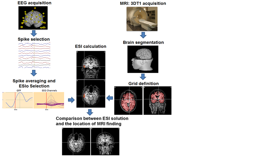
Figure 1. A schematic flux of acquisition and processing steps applied for obtaining ESI maps. The EEG data is acquired, then the IED are marked and averaged, then the ESI method is applied considering a distribution of points (GRID) within a head model estimated by the individual 3dT1 Image.
global field power (GFP) was estimated. We considered the 50% rising phase of the averaged IED presented in the GFP [17] as the spike onset (ESIo), and this was the time instant considered to calculate the ESI.
2.4. ESI Methods
We applied six different methods of solving the inverse problem. They are implemented in two different software: 1) The Neuronic Source Localizer software (Neuronic, Havana, Cuba) was used for the application of the methods Minimum Norm, LORETA and BMA. 2) The software BESA Research 6.0 (BESA, Gräfelfing, Germany) was used for applying the methods CLARA, LAURA and Equivalent Dipole (ED).
2.5. Head Modeling
The head models were done by two different software:
1) iMagic (Neuronic, Havana, Cuba) was used for preparing the head models to Neuronic Source Localizer. In this software we used the patient individual MRI for segmenting the whole brain, but the cerebellum. The segmentation of the brain in regions was based on the MNI atlas [18] and we considered 91 anatomic regions from this atlas. We defined the GRID by points 4 mm equidistant between each other, and we modeled the scalp, liquor and brain tissues as a 3 concentric spheres.
2) The software BESA MRI (BESA, Gräfelfing, Germany) was applied for modeling the head to be used by BESA Research 6.0. The patient individual MRI was segmented based on the Talairach atlas, but the brain steam and cerebellum were excluded. The GRID was defined by points 4 mm equidistant from each other and the scalp, liquor and brain tissues were modeled as a 3 concentric spheres.
The electrodes were set in the patients’ reconstructed digital scalp using the 10|10 or 10|20 position system, according to the EEG acquisition setup.
2.6. Evaluating the Results
We evaluate our results comparing the ESI maps with the abnormalities found in the patient’s MRI. We did three different comparisons: 1) calculating the Euclidian distance from the center of the lesion (CL) to the point referent to the maximum primary current density (PCD) of each method (method’s maximum, MM). These values were called CL-MM. 2) we calculated the minimum distance from the CL and the border of the ESI solution containing values higher than 50% of the method’s maximum (border of the method, BM). These values were called CL-BM. 3) We also applied the score system illustrated in the Figure 2 to quantify the solutions according to their clinical significance.
The scores could vary from 0 to 3 points and they depended on the position of the method’s solution compared to the MRI’s abnormality position as follows: 0) contralateral to the lesion; 1) ipsilateral to the lesion; 2) same or in the edge of the lesion’s lobe (lobar level) and 3) same or neighbor structure of the lesion (sub lobar level). The lesion’s region is illustrated by the red circle in the Figure 2.
3. Results
In the current paper we discuss one patient more detailed, and two more patients are presented in Supplementary Material, in order to highlight how the ESI methods can be useful for the clinical routine related to epilepsy. These cases also show how the ESI solutions are related to the mean questions discussed in this paper as the number of electrodes and its potential as an auxiliary tool in cases that have disagreement between EEG monitoring report and MRI findings. It is also important to note that the Figure 3 and Figure S1 and Figure S2 of Supplementary Material present results obtained by two different software. Therefore, they have different background colors: those from BESA are always in letters a (lesion location), b (ED), c (LAURA) and d (CLARA), and have the lighter background. The solutions obtained by the methods implemented in Neuronic Source Localizer have a dark background and are presented always in letters e (lesion location), f (BMA), g (LORETA) and h (MN). In all the images the radiological convention is assumed.
Patient #17 The MRI finding of this patient was a lesion in the right superior frontal gyrus (Figure 3(a) and Figure 3(e)). The Single Photon Emission Tomography (SPECT) indicated bilateral hyperperfusion in the superior frontal gyrus, more accentuated in the right hemisphere. However, the electroclinical evaluation based on ictal and interictal EEG events concluded that the epileptogenic region is in the left hemisphere. The ESI maps of all methods (Figure 3), but MN (Figure 3(h)) found the solution’s maximum in the neighborhood of the left superior frontal lobe.
The results of our evaluation are presented for each method applied. They are summarized in the Table 2 (location of each solution maxima) and Table 3 (CL-MM and CL-BM distances of each method).
Figure 4 groups the total score (Figure 4 left) and the results obtained by the CL-MM (4 right), with their range of variation, for each method.
The method BMA was the one with the highest score (45) and also the lowest mean CL-MM (27 mm), Figure 4 (left and right figures, respectively). Although the mean distance CL-BM of the methods LAURA (2 mm) and LORETA (10 mm) were shorter than the obtained by BMA (15 mm), their solutions were always more dispersed, overlapping many others brain structures. This is illustrated in the Figure 3, and Figure S1 and Figure S2 of Supplementary Material, (letter c for LAURA and g for LORETA). On the other hand the BMA maps were more restrict than those obtained by the other methods, which is exemplified in Figure 3(f), and also in Supplementary Material by the Figure S1(f) and Figure S2(f).
We also evaluated the percentage of solutions that mapped the structure presenting a lesion on the anatomical images of temporal and extra-temporal patients. Therefore, in order to evaluate the sensitivity of our results we assumed that maps scoring 2 or 3 points in our score system were well succeeded mapping the area indicated to surgery. This assumption is because the maps receiving 2 points are those mapping the structures on the surroundings of the lesion, and also on the premise that the surgeries generally resect the lesion’s area and its surrounding areas for a safety margin of error. Then we divided the number of succeeded maps by the total number of patients within the group, obtaining the values of sensitivity presented in Figure 5.
The BMA and Equivalent Dipole methods presented the highest value of sensitivity (86%) for temporal lobe patients (Figure 5). The BMA method also presented the highest sensitivity (50%) for the extra temporal patients. The minimum norm presented a high sensitivity value (71%) for the temporal lobe patients too. On the other hand, LAURA presented the lowest sensitivity (14%) for temporal lobe patients, and the methods LORETA, LAURA and CLARA presented no sensitivity for extra temporal patients.
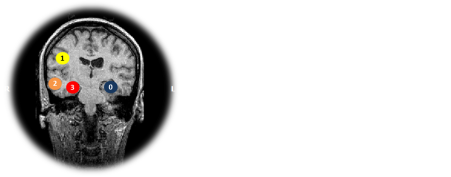
Figure 2. Score system applied for giving points based on the relation between the lesion’s location in MRI and the solutions found by ESI methods. Considering the lesion in the red circle, the scores are: 0) for method with the maxima contralateral to the lesion (blue circle), 1) for methods with maxima ipsilateral to the lesion (yellow circle), 2) for solutions with maxima in the same lobe of the lesion (orange circle), and 3) for solutions in the affected structure (red circle).
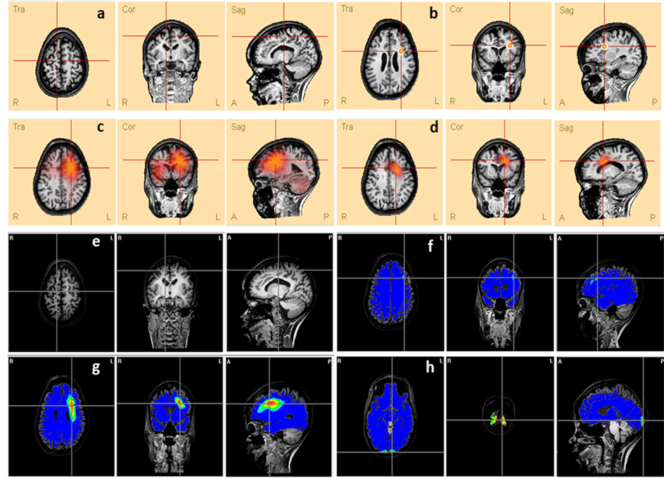
Figure 3. Comparison between the lesion (a and e) presented in patient’s #17 MRI and the ESI obtained by different methods: (b) ED, (c) LAURA, (d) CLARA, (f) BMA, (g) LORETA and (h) MN. The lines’ intersection indicates the patient’s lesion (a and e) and the maxima of each method (c, d, f, g and h). It also shows the dipole location (b).
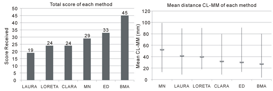
Figure 4. Evaluations results: Total score obtained for each method (left figure) and the mean distance CL-MM in millimeters and the range of results for each method (right figure).
Table 2. Anatomical location of the maxima value found by different ESI methods (R, right; L, left; ITG, inferior temporal gyrus; STG, superior temporal gyrus; MTG, middle temporal gyrus; CH, cerebellar hemisphere; MOG, middle occipital gyrus; FL, frontal lobule; Hipp, hippocampus; SMG, supra marginal gyrus; Pre-C G, pre-central gyrus; SPG, superior parietal gyrus; TP, temporal pole; IPL, inferior parietal lobule; ACG, anterior cingulate gyrus; Pos-C G, pos-central gyrus; Operc, opercula; AG, angular gyrus).
Finally, we compared the results obtained by the methods that presented the best performances (BMA and ED) applying an unpaired t-tests. We compared the mean CL-MM distance obtained by each method for in each group of patients. For neither temporal lobe nor extra-temporal lobe patients we detected differences in the distances measured.
4. Discussion
In this study we calculated ESI maps of IED from EEG data of 20 patients with epilepsy. We applied six different methods to calculate ESI maps in order to evaluate their results based on the location of MRI abnormalities. Then, we calculated Euclidian distances to measure the distances from the center of the abnormality to the max
Table 3 . CL-MM and CL-BM distances calculated for the different ESI methods (CL-MM distance from the center of the lesion to the maximum of the method; CL-BM, distance from the center of the lesion to the region containing the PCD higher than 50% of solution’s maxima; MN, Minimum Norm).
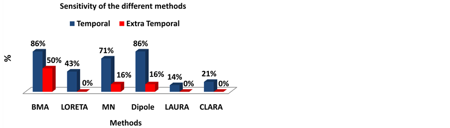
Figure 5. Sensitivity of the different ESI methods. We considered the maps that scored 2 and 3 as the well succeeded in mapping the epileptogenic region. So we divided the number of maps that scored 2 and 3 points by the total number of patients in each group (Temporal patients and extra temporal patients).
imum and the closest border of each method solution. We also applied a score system to evaluate the concordance of the maps obtained with the clinical information available. Finally we evaluated the sensitivity of each method in mapping the considered epileptogenic region.
Our results are concordant to those reported in literature for applying ESI methods in EEG data of epilepsy patients. Particularly comparing the results obtained by the equivalent dipole method to those found for others authors. For example, comparing the ED to the position of the lesion’s edge [12] [19] [20] present in MRI. In one study [11] the authors calculated the mean distance between the position of the dipole and the closest and farther border of the lesion, and the mean distances found were 5 mm (in the range of 0 to 8 mm) and 28.8 mm (in the range of 4 and 62 mm), respectively. In another study [19] the mean distance from the dipole to the closest border of the lesion was found to be 14.5 mm (in the range of 0 to 36 mm). Although the distances obtained for ED method in our study were higher (mean CL-MM of 31 mm in the range from 14 to 91 mm), we only considered the lesion’s center, disregarding the lesion extension, which sometimes was larger than an sphere of 25 mm of diameter.
The high distances obtained in some cases are also related to the few electrodes used for acquiring the EEG data. For example, the patient #2 (Supplementary Material Figure S1) had the EEG acquired in only 16 electrodes and exhibited low concordance between ESI maps and clinical information. Another example is the patient #5 that presented high distances CL-MM and CL-BM, but not for LAURA and LORETA that presented blurred maps. The patient’s #5 EEG data were acquired by 18 electrodes. There is a study [4] reporting shorter distances between the positions of a simulated source and the reconstructed source than the obtained in our results. The authors simulated the 148 electrodes-EEG signal of an electrical source within the brain and obtained maps for the methods Weighted Minimum Norm (7.29 mm), LORETA (4.20 mm) and LAURA (3.26 mm).
The sensitivities of the ESI methods presented in this study are also concordant with those reported in literature for some of the methods. Here, for example, we found sensitivities of 43% and 71% for the methods LAURA and MN when applied in temporal lobe patients’ data in the condition called as low resolution ESI (LR-ESI) in the study done by Brodbeck and colleagues [16] . In their study, the authors found a sensitivity of 67.3% for the solutions obtained by the application of the method LAURA on EEG data acquired by 19 - 29 electrodes, in temporal lobe patients. Although our assumption of successful maps was not based on surgery resection and outcome, we found highest values of sensitivity for three methods (BMA, Equivalent Dipoles and MN), but our range of electrodes used for acquiring the data was within 16 and 63 electrodes. However, our results obtained by ED and BMA were close to the results found for Brodbeck and colleagues [16] using the so-called high resolution ESI (using more than 128 electrodes to acquire the EEG data). In this situation the authors obtained a sensitivity of 91.7% using the method LAURA in temporal lobe epilepsy EEG data. Even though the methodology for comparing results with the epileptogenic area are different, our results for BMA and ED (86%) show that studies with few electrodes are also important and needed to be done. We believe that the evaluation ESI on EEG data acquired with few electrodes has its value, because methods such as BMA and ED may help to diffuse the ESI use for a more clinical environment, where few electrodes are utilized for acquiring the EEG data.
Although the t-test results did not detect differences between the mean distances measured by the methods, in none of the groups, the scores obtained by BMA mapped the structure (scoring 3 points in the suggested system) of the lesion in 8 of the 14 temporal lobe patients. On the other hand, the ED method did not score 3 points in any of the temporal lobe patients. These results support the recurrent expectations highlighted in different reviews [14] [21] about BMA potential uses in epilepsy EEG-data. Finally, we might regard the results obtained by the mean CL-BM for the BMA method, which were 13 mm for the temporal lobe patients and 20 mm for the extra temporal patients. These results are both similar to those reported in literature for other groups by applying ESI on real and simulated EEG data [4] [11] [19] .
Methodological Issues and Future Research
There are three methodological issues in this paper. The first one is related to the usage of two different software for applying ESI. Although the head modeling was not exactly the same for both ESI software, it was not our aim to compare the influence of head modeling features over the results. Our scope in this paper was to compare different methods that are clinically available in different software. Therefore, we do think that a more careful analysis should be done if the interest was to evaluate differences related to the implementation of the methods and not their applicability on the epilepsy clinical routine. The second point is about our assumption that the lesions associated to epilepsy activities were the only responsible for these activities. Hence, we considered here the damaged structure and its surrounding (neighbor structures) as the area that would be resected in a surgery. Therefore our comparisons to results reported in literature were interesting to regard the potential of applying BMA on EEG data of few electrodes, but its validation needs further work. Finally, we believe that would be interesting to have more patients with extra temporal epilepsy such as in frontal lobe, because it would be possible to evaluate the methods performance for each lobe instead to evaluate it as a single group called extra temporal patients.
As a future research, we believe that the BMA should be applied in a wider range of data, acquired with different number of electrodes to allow a comparison to the results reported in literature for other methods with more similar conditions.
5. Conclusion
We found that the application of ESI for reconstructing IED activities is sensitivity for EEG acquired by few numbers of electrodes (<63). Although our methodological conditions were not the same of other studies reported in literature, the methods BMA and ED presented high sensitivities for temporal lobe epilepsy patients (86%). The BMA method also obtained the lowest mean CL-MM distance and the third lowest CL-BM, but presented solutions restricted to few structures and more representative than those obtained for the other methods. Finally, we believe that the BMA method needs to be explored in wider sets of data, including more extratemporal lobes patients and also EEG data acquired with different number of electrodes.
Acknowledgements
We thank the São Paulo Research Foundation for the financial support.
References
- Helmholtz, H. (1853) UebereinigeGesetze der Vertheilungelektrischer Ströme in körperlichen Leiternmit Anwendung auf die thierisch-elektrischen Versuche. Annalen der Physik und Chemie, 9, 211-233. http://dx.doi.org/10.1002/andp.18531650603
- Scherg, M. (1990) Fundamentals of Dipole Source Potential Analysis. In: Grandori, F. and Romani, G., Eds., Auditory Evoked Electric and Magnetic Fields. Topographic Mapping and Functional Localization. Advances in Audiology, 6, Basel, Karger, 40-69.
- Hämäläinen, M.S. and Ilmoniemi, R.J. (1984) Interpreting Measured Magnetic Fields of the Brain: Estimates of Current Distributions. Technical Report TKK-FA559, Helsinki University of Technology, Espoo.
- Pascual-Marqui, R.D., Michel, C.M. and Lehmann, D. (1994) Low Resolution Electromagnetic Tomography: A New Method for Localizing Electrical Activity in the Brain. International Journal of Psychophysiology, 18, 49-65. http://dx.doi.org/10.1016/0167-8760(84)90014-X
- Menendez, R.G.P., Gonzalez, S.L.A., Lantz, G., Michel, C.M. and Landis, T. (2001) Noninvasive Localization of Electromagnetic Epileptic Activity. I. Method Descriptions and Simulations. Brain Topography, 14, 131-137. http://dx.doi.org/10.1023/A:1012944913650
- BESA (2010) Research Tutorial 4: Distributed Source Imaging. http://besa.de/tutorials/hands_on,Germany
- Trujillo, N.J.B., Vázquez, E. and Valdés, P.A.S. (2004) Bayesian Model Averaging in EEG/MEG Imaging. NeuroImage, 21, 1300-1319. http://dx.doi.org/10.1016/j.neuroimage.2003.11.008
- Laehy, R., Mosher, J.C. and Phillips, J.W. (1996) A Comparative Study of Minimum Norm Methods for MEG Imaging. Proceedings of the Tenth International Conference on Biomagnetism, Biomag’96, Santa Fe, 247-277.
- Menendez, G.P.R. and Gonzalez S.L.A. (2002) Comparison of Algorithms for the Localization of Focal Sources: Evaluation with Simulated Data and Analysis of Experimental Data. International Journal of Bioelectromagnetism (Online Journal).
- Rusiniak, M., Lewandowska, M., Wolak, T., Pluta, A., Milner, R., Ganc, M., Wlodarczyk, A., Senderski, A., Sliwa, L. and Skarzyński, H. (2013) A Modified Oddball Paradigm for Investigation of Neural Correlates of Attention: A Simultaneous ERP-fMRI Study. MAGMA, 26, 511-526. http://dx.doi.org/10.1007/s10334-013-0374-7
- Merlet, I. and Gotman, J. (1999) Reliability of Dipole Models of Epileptic Spikes. Clinical Neurophysiology, 110, 1013-1028. http://dx.doi.org/10.1016/S1388-2457(98)00062-5
- Krings, T., Chiappa, K.H., Cuffin, B.N., Buchbinder, B.R. and Cosgrove, G.R. (1998) Accuracy of Electroencephalographic Dipole Localization of Epileptiform Activities Associated with Focal Brain Lesions. Annals of Neurology, 44, 76-86. http://dx.doi.org/10.1002/ana.410440114
- Ebersole, J.S. (1997) Defining Epileptogenic Foci: Past, Present, Future. Journal of Clinical Neurophysiology, 14, 470-483. http://dx.doi.org/10.1097/00004691-199711000-00003
- Michel, C.M., Menendez, G.P.R., Lantz, G., Gonzalez S.L.A., Spinelli, L., Blanke, O., Landis, T. and Seeck, M. (1999) Spatiotemporal EEG Analysis and Distributed Source Estimation in Presurgical Epilepsy Evaluation (Review). Journal of Clinical Neurophysiology, 16, 239-266. http://dx.doi.org/10.1097/00004691-199905000-00005
- Fuchs, M., Wagner, M., Kohler, T. and Wischmann, H.A. (1999) Linear and Nonlinear Current Density Reconstructions (Review). Journal of Clinical Neurophysiology, 16, 267-295. http://dx.doi.org/10.1097/00004691-199905000-00006
- Brodbeck, V., Spinelli, L., Lascano, A.M., Wissmeier, M., Vargas, M.I., Vulliemoz, S., Pollo, C., Schaller, K., Michel C.M. and Seeck, M. (2011) Electroencephalographic Source Imaging: A Prospective Study of 152 Operated Epileptic Patients. Brain, 134, 2887-2897. http://dx.doi.org/10.1093/brain/awr243
- Lantz, G., Spinelli, L., Seeck, M., Menendez, G.P.R., Sottas, C.C. and Michel, C.M. (2003) Propagation of Interictal Epileptiform Activity Can Lead to Erroneous Source Localizations: A 128-Channel EEG Mapping Study. Journal of Clinical Neurophysiology, 20, 311-319. http://dx.doi.org/10.1097/00004691-200309000-00003
- Collins, D.L. (1994) 3D Model-Based Segmentation of Individual Brain Structures from Magnetic Resonance Imaging Data. Ph.D. Thesis, McGill University, Montreal.
- Huppertz, H.J., Hoegg, S., Sick, C., Lücking, C.H., Zentner, J., Schulze-Bonhage, A. and Kristeva-Feige, R. (2011) Cortical Current Density Reconstruction of Interictal Epileptiform Activity in Temporal Lobe Epilepsy. Clinical Neurophysiology, 112, 1761-1772. http://dx.doi.org/10.1016/S1388-2457(01)00588-0
- Michel, C.M., Lantz, G., Spinelli, L., Menendez, G.P.R., Landis, T. and Seeck, M. (2004) 128-Channel EEG Source Imaging in Epilepsy: Clinical Yield and Localization Precision. Journal of Clinical Neurophysiology, 21, 71-83. http://dx.doi.org/10.1097/00004691-200403000-00001
- Grech, R., Cassar, T., Muscat, J., Camilleri, K.P., Fabri, S.G., Zervakis, M., Xanthopoulos, P., Sakkalis, V. and Vanrumste, B. (2008) Review on Solving the Inverse Problem in EEG Source Analysis. Journal of NeuroEngineering and Rehabilitation, 5, 25. http://dx.doi.org/10.1186/1743-0003-5-25
Supplementary Material
Patient #2 This patient presented a lesion in the posterior right portion of the parietal lobe (Figure S1(a) and Figure S1(e)), visible in the MRI. None of the ESI solutions overlapped the lesion, actually all the methods, but the MN (Figure S1(h)), found solutions only ipsilateral to the lesion.
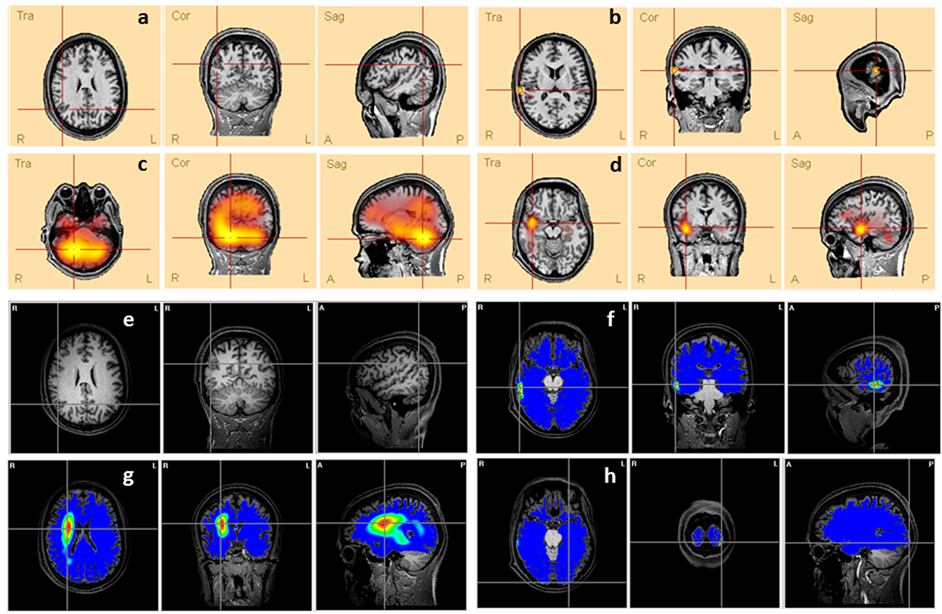
Figure S1. Comparison between the lesion (a and e) presented in patient’s #2 MRI and the ESI obtained by different methods: (b) ED, (c) LAURA, (d) CLARA, (f) BMA, (g) LORETA and (h) MN. The lines’ intersection indicates the patient’s lesion (a and e) and the maxima of each method (c, d, f, g and h). It also shows the dipole location (b).
Patient #13 The MRI presented a relatively large lesion in the superior portion of the left occipital lobe (Figure S2(a) and Figure S2(e)). The electroclinical evaluation had shown paroxysms in the P3 and PO3 electrodes. The ESI solutions found by the methods ED (Figure S2(b)), CLARA (Figure S2(d)) and BMA (Figure S2(f)) are coherent to the clinical data, but only the BMA’s map was found in the same brain region of the lesion.
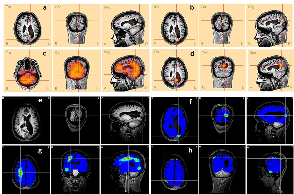
Figure S2. Comparison between the lesion (a and e) presented in patient’s #13 MRI and the ESI obtained by different methods: (b) ED, (c) LAURA, (d) CLARA, (f) BMA, (g) LORETA and (h) MN. The lines’ intersection indicates the patient’s lesion (a and e) and the maxima of each method (c, d, f, g and h). It also shows the dipole location (b).