Journal of Biomedical Science and Engineering
Vol.7 No.5(2014), Article ID:45037,10 pages DOI:10.4236/jbise.2014.75031
A Model Metabolic Cycle Simulated with the Mathematica Program
Víctor García-Herrero, Francisco López-Cánovas, Antonio Sillero*
Departamento de Bioquímica, Facultad de Medicina, Instituto de, Investigaciones Biomédicas Alberto Sols UAM/CSIC, Madrid, Spain
Email: *antonio.sillero@uam.es
Copyright © 2014 by authors and Scientific Research Publishing Inc.
This work is licensed under the Creative Commons Attribution International License (CC BY).
http://creativecommons.org/licenses/by/4.0/


Received 2 March 2014; revised 5 April 2014; accepted 13 April 2014
ABSTRACT
A system of differential equations has been used to simulate a model metabolic cycle, containing only one initial substrate and 8 irreversible enzymes. The metabolic course of the intermediates (products/substrates) was also explored in different situations: changes in the kinetic constants of one of the enzymes of the cycle; introduction of one reversible step; consecutive increments in the Km values of each enzyme of the cycle and the presence of two initial substrates. A decrease or an increase in the Km value of one of the enzymes of the cycle promotes a decrease or an increase in the steady state level of its own substrate, respectively; by the contrary, a decrease or an increase in the Vmax value promotes, respectively, an increase or a decrease in the stationary level of the corresponding substrate. A comparison between a linear and a cyclic metabolic pathway is also presented.
Keywords:Metabolic Pathways, Metabolic Cycle, Mathematical Simulations, Differential Equations

1. Introduction
The rate of appearance and disappearance of the intermediate substrates of a linear metabolic pathway (here named as their profiles) catalyzed by 5 or 7 consecutive irreversible enzymes was previously reported, simulated with the help of the Mathematica Program [1] . These profiles presented different shapes depending on both the Vmax and Km values of the enzymes involved, and on the amount of the initial substrate of the pathway. In the case of a linear pathway, it was supposed that the initial substrate was consumed and totally converted into a final product with the concomitant appearance and disappearance of the intermediate substrates of the pathway [2] .
It seemed to us that a similar approach could be followed to analyze a metabolic cycle where continuous and consecutive transformations among different substrates catalyzed by different enzymes are taking place. It is common knowledge that the biochemical machinery of a cell, or of any organism as a whole, is partially based on the occurrence of linear, branched and circled pathways, interrelated among them by metabolic crossroads and by diverse control mechanisms [3] -[7] . The resulting panorama is so complex that, both experimental and mathematical treatments [2] [8] [9] might be necessary to apprehend even particular zones of this complex organization.
Whereas simulations of linear pathways are widely documented [2] , similar studies on metabolic cycles are, to our knowledge, rather scarce in spite of the crucial relevance of some of these cycles in biochemical processes. In this work, diverse aspects of a particular example of a model metabolic cycle composed of 8 enzymes have been explored. Similar studies could be performed with cycles composed by a different number of substrates/ enzymes. The effect of changing the kinetic constants (Vmax and Km values) of one or several enzymes of the cycle has been also examined. The Vmax and Km values are two parameters widely used in the study of enzyme kinetics [3] [4] . As shown below, the metabolic situation generated by a group of enzymes acting linearly or forming a cycle presents both similar and different metabolic consequences.
2. Experimental Procedures
Computation
The Mathematica Program 9.0 [10] was used throughout this work to solve the differential equations describing metabolic pathways (see Table 1), with the following main commands: derivatives, D[f(x), x]; plot representations, Plot[f(x), x, xmin, xmax]; solution of a system of differential equations, NDSolve [eqns, vars]. In the Mathematica Program: a’[t], b’[t], etc., correspond to da/dt, db/dt, etc.; one space is equivalent to a multiplication sign; x = y is an imperative statement that actually causes an assignment to be done; x = y merely tests whether x and y are equal and causes no explicit action. The model cycle containing 8 substrates is schematically represented in Figure 1, and its mathematical treatment listed in Table 1.

Table 1. Mathematica protocol used to simulate a cyclic or linear pathway, with potential changes in enzyme kinetic constants. More details are in Figure 1 and in the Text.
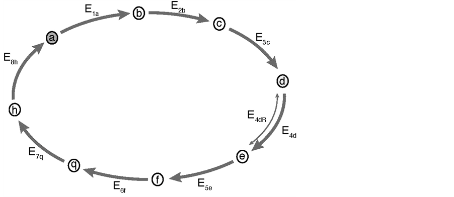
Figure 1. Biochemical cycle, Schematic representation of a biochemical cycle composed of 8 different substrates a- > b- > c- > d- > e- > f- > q- > h- > a and by 8 enzymes: E1a, E2b, E3c, E4d, E5e, E6f, E7q, E8h. The transformation of this cyclic into a linear pathway is mathematically obtained by simply eliminating enzyme E8h (i.e. E8h = 0) from the cycle. In this case the transformation h- > a does not take place, and (a) and (h) are then the first and the last substrates of the linear pathway, respectively. Note as: i) because of problems with the correct recognition of the letter “g” by the Mathematica Program, “q” replaces letter “g” in the sequence of substrates of the cycle; ii) the substrates will be indicated in parentheses, hence (a) is simultaneously the first and the last substrate of the cycle; iii) the enzymes (E) are numbered with two sub-indexes: indicating their order in the reaction (from 1 to 8) and the corresponding substrate. For example E5e, stands for the fifth enzyme of the sequence acting on substrate (e); iv) substrate (a) is marked in the figure to indicate that it is the first substrate of the cycle; v) in two particular cases: substrate (a) and (d) were considered as initial substrates of the cycle, and step 4 was considered reversible.
To facilitate the presentation of the model (Figure 1), the enzymes (E) are named, in general, as E1 to E8 or, more specifically, as E1a, E2b, E3c, E4d, E5e, E6f, E7q, E8h; the sub indexes representing the order (from 1 to 8) and the sequence of the reactions (from a to h): a- > b- > c- > d- > e- > f- > q- > h- > a; because a problem of adequate recognition of letter “g” by the Mathematica Program, this letter was replaced by “q” as a substrate of the cycle
(Figure 1). In one particular case, the reaction catalyzed by enzyme E4d was considered reversible and the enzyme named as E4dR, with the following kinetic constants: in the forward (f) and reverse direction (r), Km4f, Vmax4f , Km4r, Vmax4r (Table 1). The equation velocity v4N (N, for Net velocity) between the two substrates (d and e) is shown in Table 1 and in Equation (2) (see below). Note as: i) when convenient, the name of the substrates are indicated in the text, between brackets; ii) the substrate (a) is simultaneously the initial and the final substrate of the cycle.
The following parts can be considered in Table 1: 1) equations of the actual velocities of the enzymes E1 to E8, (named from v1 to v8), expressed with the classical Michaelis-Menten equations: maximal velocities (Vmax) are indicated as Vmax1 to Vmax8 and Km values as Km1 to Km8; the sequence of the reactions are indicated in Figure 1; 2) actual values for the kinetic constants for each enzyme; the value assigned to all the constants in the control pathway is the unity; 3) differential equations used to calculate the changes in the concentration of the substrates along the reaction time, together with the initial conditions, unknowns be solved and time of reaction; 4) the statements required for the Mathematica Program to solve the differential equations shown above, and to present the graph shown both in Figure 2, panel A.
The variants of the cycle shown below are easily executed following the commands in Table 1, only by changing the values of the kinetic constants as shown in parts 2 and 3).
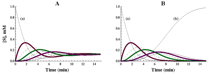
Figure 2. Representation of a cyclic pathway (A) and of a linear irreversible pathway (B), simulated with the Mathematica Program. In panel A, the specifications consigned in Table 1 were strictly followed. For the drawing of panel B, Table 1 was essentially modified as follows: the enzyme E8h was eliminated (i.e. v8 = 0) and hence the concentration of (a) considered for the calculations of the differential equations was a’ [12] = v8 − v7 = −v7. In A and B the kinetic values of the concerned enzymes were the unity for both the Vmax and Km values.
3. Results and Discussion
3.1. A Model Cycle Primed with Only One Initial Substrate and Composed of 8 Enzymes Comparison with a Similar, but Linear, Irreversible Pathway
After applying the differential equations described in Table 1, the plot represented in Figure 2, A was obtained. As soon as the simulation is initiated, the concentration of the initial substrate (a) starts to decrease and is promptly (min 0 to 8 of reaction) converted to changes in all the intermediates of the cycle. As the 8 enzymes of the control cycle have the same kinetic constants (Vmax = 1 micromole/min; Km = 1 mM), it is expected that the amount of the initial substrate (a) is equally distributed among the 8 substrates of the cycle when the steady state is reached: 1/8 = 0.125 mM (Figure 2(A)). The Mathematica commands (Table 1) allow different times of reaction (see part 3), what can be used for different purposes. If the steady state is expected to be reached (and examined) at longer incubation times, a poor vision of the initial profiles of the reaction could be obtained. By contrast, if the objective is to examine the initial steps, shorter reaction times are more convenient. In this work, a compromise with respect to the reaction time (from 0 to 15 min) was used to get a good view on both the initial and the final stages of the reaction.
As an illustrative complement to this cycle, a linear irreversible pathway composed of 7 substrates and 7 enzymes was mathematically simulated and presented in Figure 2, panel B. The change of a cyclic to a linear pathway was obtained by simply eliminating enzyme E8h, which transforms the last substrate of the cycle (h) into the first one (a), (what is equivalent to make v8 = 0). With this modification, the first substrate (a) is totally transformed into the end product (h) of the now linear pathway. As the kinetic characteristics of the enzymes of the cyclic and linear pathways are identical (Km and Vmax values are equal to 1 the comparison between both pathways is easily visualized. Initially, the profiles of the components of both pathways follow a similar course, but diverge when they tend to reach quite different steady states (compare panels A and B in Figure 2).
3.2. Influence of Changing the Vmax or the Km Values of One, or Several Enzyme(s) in a Metabolic Cycle
Changes in the kinetic parameters were firstly simulated on the enzyme E4d; its Km value was modified from 1 mM (control, Figure 2(A)) to 0.3 mM (Figure 3(A)), or to 3 mM (Figure 3(B)). The decrease (Figure 3(A)) or the increase (Figure 3(B)) of the Km value of the enzyme E4d promoted a decrease, or an increase, respectively, in the steady state concentration of its substrate (d) (as marked in Figure 3(A) and Figure 3(B)), whereas, the other substrates (a, b, c, e, q, h) of the cycle reached almost similar steady state concentrations (Figure 3(A) and Figure 3(B)).
The influence of changing the Vmax value of the same enzyme (E4d) was also explored. The profiles of the cycle when the Vmax value was changed from 1 to 0.3 micromole/min or from 1 to 3 micromole/min are represented in Figure 3(C) and in Figure 3(D), respectively. As a consequence of these changes, the proper
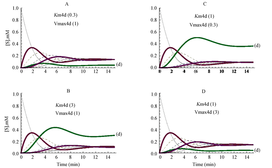
Figure 3. Influence of changing the Vmax or the Km values of only one enzyme (E4d) of the cycle. The Km value of E4d was changed from the standard value of 1 to 3 mM (panel A) or to 0.3 mM (panel B), and the reaction followed up to the metabolites approaching their steady state level. The figures between brackets correspond to the values for Km4d (mM) and Vmax4d (micromole/min), respectively.
substrate (d) of the enzyme reached comparatively higher and lower steady state levels, respectively, whereas the other components of the cycle reached similar stationary levels in Figure 3, panels C and D.
Comparatively results were obtained when similar changes in the Km or Vmax values were simulated in any of the other enzymes of the cycle (results not shown); a metabolic cycle operates as a functional unit, and similar changes in different enzymes promote similar overall changes in the cycle.
A diversity of alternatives, obtained by increasing or decreasing the Km or the Vmax values of several, consecutive or alternating enzymes, can be simulated by simply changing the adequate parameters in Table 1 (not shown). As an example of the versatility of the Program for the handling of the cycle, only the results promoted by simultaneous modifications of the Km values of the 8 enzymes of the cycle are shown in panels A and B of Figure 4. In this example the Km modified values are indicated between brackets: E1a (0.2); E2b (0.4); E3c (0.6); E4d (0.8); E5e (1.0); E6f (1.2); E7q (1.6); E8h (1.8). Two scales for the y-axis, 1 and 0.5 mM, were used in panels A and B, respectively. In panel B it is clearly appreciated as these changes in the Km values promoted different steady state levels for each one of the substrates of the cycle (Figure 4).
3.3. Reversibility of One of the Reactions in a Model Cycle
A different type of simulation was now explored by introducing a different enzyme (named as E4dR) (Figure 1) catalyzing the reversible reaction (1), with the equation velocity (𝑣4N) detailed in (2) and in part Table 1, part 1)).
 (1)
(1)
 (2)
(2)
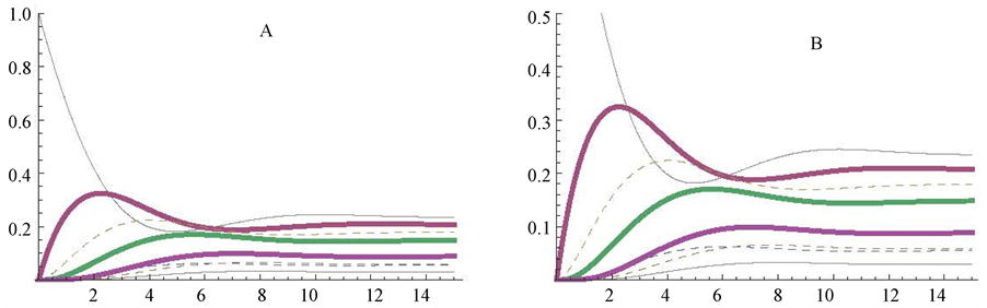
Figure 4. Different Km values applied to the 8 enzymes of the cycle. The Km values (mM) are indicated between brackets: E1a (0.2); E2b (0.4); E3c (0.6); E4d (0.8); E5e (1.0); E6f (1.2); E7q (1.6); E8h (1.8). Two scales for the y-axis, 1 and 0.5 mM, were used in panels A and B, respectively. In panel B it is clearly appreciated that the changes in the Km values promoted different steady state levels for each one of the substrates of the cycle.
The Mathematica program detailed in Table 1 is so arranged that a simple replacement of v4 by v4N in part 3 of Table 1 (one of the commands of NDSolve) is enough to simulate this reversible step. Nevertheless it is convenient to note that all the kinetic constants (Km4f; Vmax4f; Km4r and Vmax4r) are settled at the value of 1.The operator can modify these values at will, to obtain modified values for E4dR. In this work we have considered only the following alternatives in the forward (f) direction d- > e: Km4f with values of: 0.1, 0.3 and 3 mM, (Figure 5, panels A, B, C, respectively); Vmax4f with values of: 0.1, 0.3 and 3 micromole/min, (Figure 5, panels D, E, F, respectively). The profiles in Figure 5, panels B, C, D, E and F can be compared with those of the control cycle (Figure 2(A)): i) the lowering of the Vmax4f value tends to increase the stationary level of (d) (Figure 5, D): this level is around 0.8 mM, what implies an almost complete transformation of the initial substrate (a = 1 mM) into substrate (d = 0.8 mM); ii) concerning changes in the Km4f values, higher values of this parameter convey higher steady state levels of the substrate (d) (around 0.5 mM) (Figure 5(C)), and lower Km4f values elicit a significant decrease in the stationary level of (d) t (Figure 5(A)).
3.4. Insertion of Two Initial Substrates in the Cycle
Up to now, substrate (a) was considered as the first and unique initial substrate of the control cycle. To approach a different example, substrates (a) and (d) were considered initiating simultaneously the pathway (Figure 6). The direction of the cycle is as indicated in Figure 1, and metabolite (a) is still considered as the very first initial substrate. To better appreciated the profiles of substrates (a) and (d), two different initial concentrations were theoretically considered, 1 and 1.5 mM, respectively; here, only the kinetic constants corresponding to enzyme E4d were modified (Figure 6). The control profiles obtained with Vmax and Km values equal to 1 are represented in Figure 6(A). Those obtained for Km values settled at 0.3, 1 and 3 mM are represented in Figure 6(A), Figure 6(B) and Figure 6(C), respectively; those obtained for Vmax values of 0.3, 1 and 3 micromole/min are represented in Figure 6(E) and, Figure 6(A), respectively.
4. Concluding Remarks
The profiles of the intermediate metabolites of irreversible linear pathways were previously simulated with a system of differential equations [1] . In the present work, metabolic cycles have been approached. The transformation of a linear into a cyclic pathway was generated by adding a supplementary enzyme (E8h) catalyzing the synthesis of the initial substrate from the end product of the linear pathway [1] (Figure 1, Table 1). The cycle was firstly simulated in the presence of only one substrate (1 mM). Time course profiles can be grossly considered in two parts: in a first time-window (from 0 to around 8 min), a rapid transformation of the first substrate into the other components of the cycle takes place; after around 10 min, all the intermediates tend to reach a steady state situation. For that reason, a simulation of 15 min was chosen to glance all the reaction steps. If the enzymes of the cycle have identical kinetic constant values (as in the control cycle), the initial substrate is equally distributed among all the components (substrates/products) of the cycle: (1/8 = 0.125 mM).
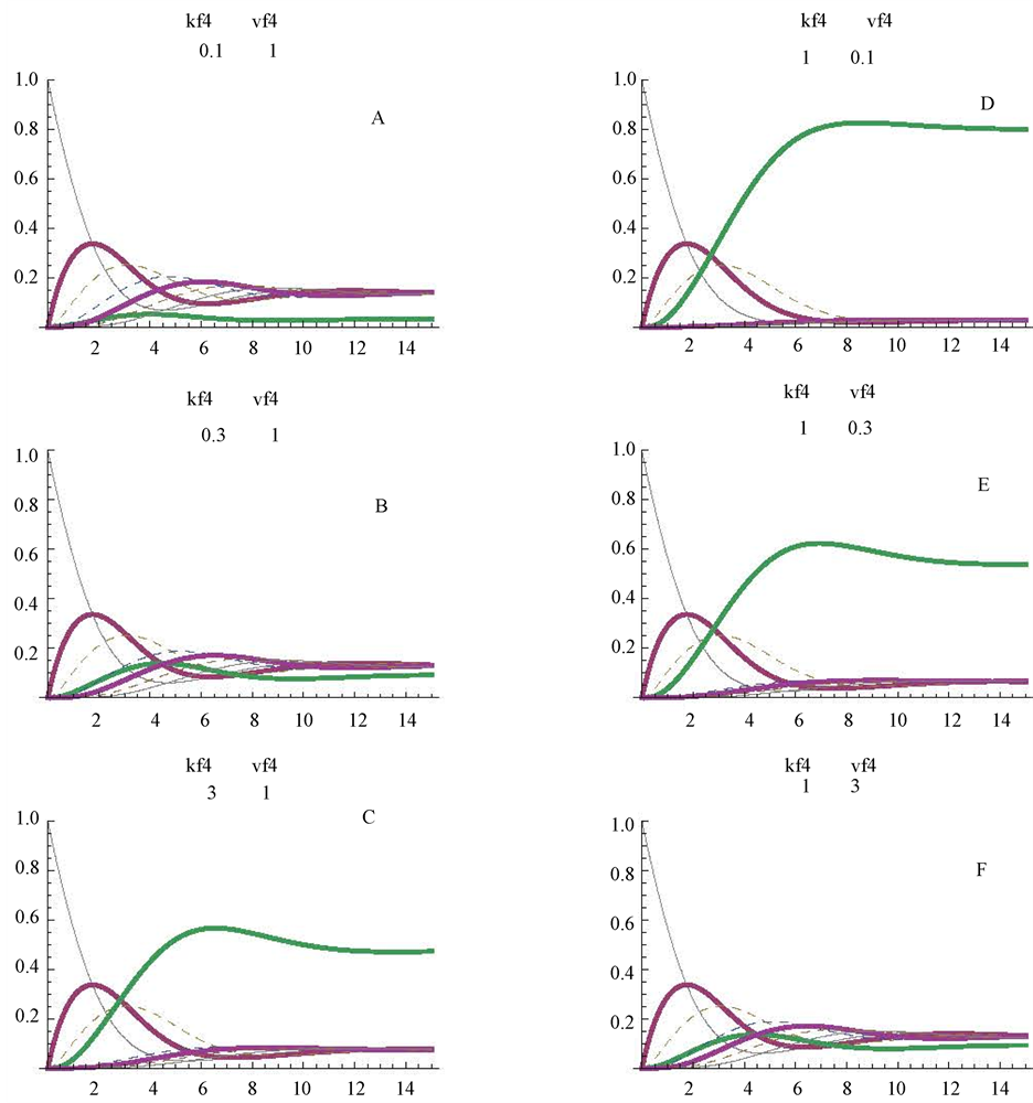
Figure 5. Reversibility of one of the step (E4dR) of the cycle (see also Figure 1). The changes were simulated only in the forward direction, with Km4f values of 0.1, 0.3 and 3 mM (panels A, B, and C respectively). The profiles obtained with Vmax4f values of 0.1, 0.3 and 3 micromoles/min are shown in panels D, E. and F, respectively. The figures between brackets, in the upper part of the panels, correspond to the values for the Km4f (mM) and Vmax4f (micromoles/min), respectively.
Illustrative results can be obtained by modifying the kinetic constants of the cycle enzymes. In general, increasing the Km and/or decreasing the Vmax values of any of the enzyme of the cycle, promoted an increase in the steady state level of the corresponding substrate.
The performance of the cycle was also tested considering three different additional conditions: i) reversibility of the reaction catalyzed by one enzyme (E4dR) (Figure 5); ii) consecutive increments in the Km values of the eight enzymes of the cycle (Figure 4) and iii) presence of two initial substrates (a) and (d) (Figure 6).
Linear pathways are present in most of the reactions involved in the metabolic and regulatory networks of the cell. Probably for this reason, mathematical simulation of these pathways has been preferentially approached
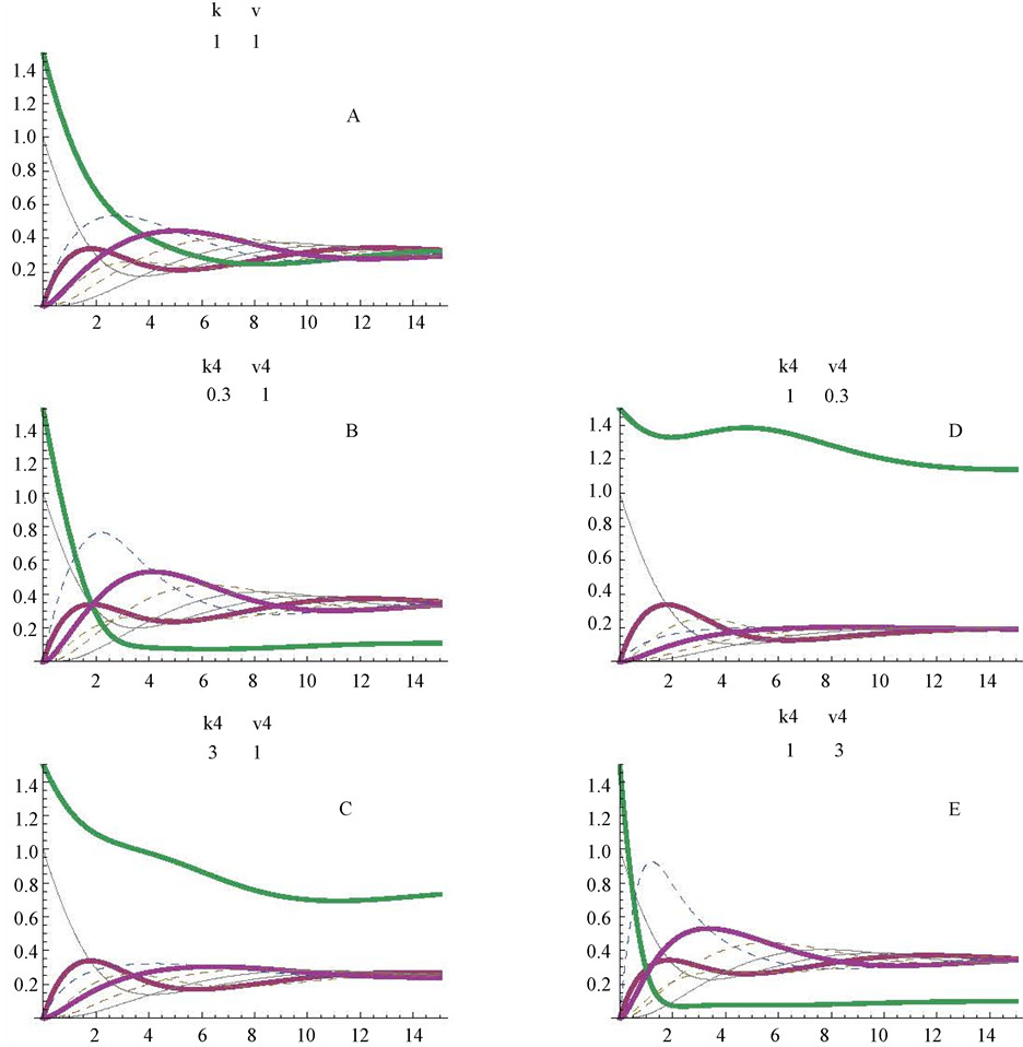
Figure 6. Simulation of a cycle with two initial substrates (a and d) and with changes in the Km and Vmax values in one of the enzymes (E4d) of the cycle. The profiles obtained at Km4d values of 1, 0.3 and 3 mM are shown in panels A, B and C; those obtained at Vmax4f values of 1, 0.3 and 3 micromoles/min are in panels A, D and E. Figures between brackets, in the upper part of the panels, correspond to the values for Km4f (mM) and Vmax4f (micromoles/min), respectively for enzyme E4d. figures under k and v applied to the corresponding values of all other enzymes of the cycle.
([2] [5] -[8] [11] ). Cyclic pathways, of similar pivotal importance, have attracted a minor number of these studies with the exception of the classical Krebs/glyoxylate ([12] -[17] ) and urea cycles ([18] -[20] ). In addition, there are a considerable number of metabolic networks, that include both linear and cyclic pathways, that could be viewed as encompassing a bigger cycle, as is the case of the functional unit formed by glycolysis, gluconeogenesis, Krebs and pentose pathway cycles ([21] [22] ). On certain occasions, these works are difficult to be followed by researchers other than those with a specific background on these topics.
In our view, and as far as Mathematica or other similar programs are available, we have tried to present a comprehensible and interactive model of a biochemical cycle that can be easily modified and reproduced by simply following the commands presented in Table 1.
Acknowledgements
We thank Javier Pérez for very helpful drawing assistance and Antonio Sillero Perles for technical assistance; María Antonia Günther Sillero and José Gonzalez Castaño for helpful comments on the manuscript, and Francisco Pérez-Zúñiga for bringing in contact VG-H and AS. VG-H is a second year student in the School of Mathematics, Complutense University of Madrid. FL-P is a second year MIR (Internal Medical Resident) in the Psychiatric Service, Hospital La Paz, Madrid. This investigation was supported by Grant BFU2009-08977.
References
- López-Cánovas, F.J., Gomes, P.J. and Sillero, A. (2013) Mathematica Program: Its Use to Simulate Metabolic Irreversible Pathways and Inhibition of the First Enzyme of a Metabolic Pathway as Visuaized with the Reservoir Model. Computers in Biology and Medicine, 42, 853-864. http://dx.doi.org/10.1016/j.compbiomed.2013.04.003
- Voet, D. and Voet, J.G. (2004) Biochemistry, XV +1591, 482-493.
- Cleland, W.W. (1970) Steady State Kinetics in the Enzymes. 3rd Edition, Academic Press, New York, 1-65.
- Krauss, M., Schaller, S., Borchers, S., Findelsen, R., Lippert, J. and Kuepfer, L. (2012) Integrating Cellular Metabolism into a Multiscale Whole-Body Model. PLOS Computational Biology, 8, e1002750. http://dx.doi.org/10.1371/journal.pcbi.1002750
- Fell, D. (1997) Understanding the Control of Metabolism. Portland Press; Distributed by Ashgate Pub. Co. in North America, London; Miami Brookfild, VT.
- Segel, I.H. (1975) Enzyme Kinetics: Behavior and Analysis of Rapid Equilibrium and Steady State Enzyme Systems. Wiley, New York.
- Klipp, R., Herwig, R., Kowald, A., Wierling, C. and Lehrach, H. (2005) System Biology in Practice. Wiley-VCH Verlag GmbH &Co, Winheim (FRG). http://dx.doi.org/10.1002/3527603603
- Alberty, R.A. (2011) Enzyme Kinetics. Rapid-Equilibrium Applications of Mathematica, Hoboken. http://dx.doi.org/10.1002/9780470940020
- Alon, U. (2006) An Introduction to System Biology. Design Principles of Biological Circuits. CRC Pres, Taylor & Francis Group, London.
- Wolfram, S. (2013) Wolfram Mathematica Tutorial Collection. http://www.wolfram.com/learningcenter/tutorialcolection
- Bisswanger, H. (2004) Enzyme Kinetics. Principle and Methods, Wiley-VCH, Weinheim (FRG).
- Albe, K.R. and Wright, B.E. (1992) Systems Analysis of the Tricarboxylic Acid Cycle in Dictyostelium Discoideum. II. Control Analysis. Journal of Biological Chemistry, 267, 3106-3114.
- Oliveira, J.S., Bailey, C.G., Jones-Oliveira, J.B., Dixon, D.A., Gull, D.W. and Chandler, M.L. (2003) A Computational Model for the Identification of Biochemical Pathways in the Krebs Cycle. Journal of Computational Biology, 10, 57- 82. http://dx.doi.org/10.1089/106652703763255679
- Wu, F., Yang, F., Vinnakota, K.C. and Beard, D.A. (2007) Computer Modeling of Mitochondrial Tricarboxylic Acid Cycle, Oxidative Phosphorylation, Metabolite Transport, and Electrophysiology. Journal of Biological Chemistry, 282, 24525-24537. http://dx.doi.org/10.1074/jbc.M701024200
- Nazaret, C., Heiske, M., Thurley, K. and Mazat, J.P. (2009) Mitochondrial Energetic Metabolism: A Simplified Model of TCA Cycle with ATP Production. Journal of Theoretical Biology, 258, 455-464. http://dx.doi.org/10.1016/j.jtbi.2008.09.037
- Amador-Noguez, D., Feng, X.J., Fan, J., Roquet, N., Rabitz, H. and Rabinowitz, J.D. (2010) Systems-Level Metabolic Flux Profiling Elucidates a Complete, Bifurcated Tricarboxylic Acid Cycle in Clostridium Acetobutylicum. Journal of Bacteriology, 192, 4452-4461. http://dx.doi.org/10.1128/JB.00490-10
- Smith, A.C. and Robinson, A.J. (2011) A Metabolic Model of the Mitochondrion and Its Use in Modelling Diseases of the Tricarboxylic Acid Cycle. BMC Systems Biology, 5, 102. http://dx.doi.org/10.1186/1752-0509-5-102
- Bachmann, C. and Colombo, J.P. (1981) Computer Simulation of the Urea Cycle: Trials for an Appropriate Model. Enzyme, 26, 259-264.
- Morris Jr., S.M. (2002) Regulation of Enzymes of the Urea Cycle and Arginine Metabolism. Annual Review of Nutrition, 22, 87-105. http://dx.doi.org/10.1146/annurev.nutr.22.110801.140547
- Maher, A.D., Kuchel, P.W., Ortega, F., de Atauri, P., Centelles, J. and Cascante, M. (2003) Mathematical Modelling of the Urea Cycle. A Numerical Investigation into Substrate Channelling. European Journal of Biochemistry, 270, 3953- 3961. http://dx.doi.org/10.1046/j.1432-1033.2003.03783.x
- Sillero, A., Selivanov, V.A. and Cascante, M. (2006) Pentose Phosphate and Calvin Cycles: Similarities and ThreeDimensional Views. Biochemistry and Molecular Biology Education, 34, 275-277. http://dx.doi.org/10.1002/bmb.2006.494034042627
NOTES

*Corresponding author.