Journal of Biomedical Science and Engineering
Vol. 5 No. 7 (2012) , Article ID: 20533 , 12 pages DOI:10.4236/jbise.2012.57049
Fully automatic identification and discrimination of sperm’s parts in microscopic images of stained human semen smear
![]()
1Department of Biomedical Engineering, Shahed University, Tehran, Iran
2Center of Operations Research University Institute Miguel Hernández University of Elche, Elche, Spain
Email: bijar@shahed.ac.ir, a.penalver@umh.es, Mikaili@shahed.ac.ir, khayati@shahed.ac.ir
Received 5 May 2012; revised 12 June 2012; accepted 28 June 2012
Keywords: Sperm; Segmentation; Rotating Calipers; Bayesian Classification; Entropy Based EM Algorithm; Structural Similarity Index (SSIM); Entropy
ABSTRACT
In the last years, digital image processing and analysis are used for computer assisted evaluation of semen quality with therapeutic goals or to estimate its fertility by means of spermatozoid motility and morphology. Sperm morphology is assessed routinely as part of standard laboratory analysis in the diagnosis of human male infertility. Nowadays assessments of sperm morphology are mostly done based on subjective criteria. In order to avoid subjectivity, numerous studies that incorporate image analysis techniques in the assessment of sperm morphology have been proposed. The primary step of all these methods is segmentation of sperm’s parts. In this paper, we have proposed a new method for segmentation of sperm’s Acrosome, Nucleus, Mid-piece and identification of sperm’s tail through some points which are placed on the sperm’s tail, accurately. These estimated points could be used to verify the morphological characteristics of sperm’s tail such as length, shape and etc. At first, sperm’s Acrosome, Nucleus and Mid-piece are segmented through a method based on a Bayesian classifier which utilizes the entropy based expectation–maximization (EM) algorithm and Markov random field (MRF) model to obtain and upgrade the class conditional probability density function (CCPDF) and the apriori probability of each class. Then, a pixel at the end of sperm’s Mid-piece, is selected as an initial point. To find other pixels which are placed on the sperm’s tail, structural similarity index (SSIM) is used in an iterative scheme. In order to stop the algorithm automatically at the end of sperm’s tail, local entropy is estimated and used as a feature to determine if a point is located on the sperm’s tail or not. To compare the performance of the proposed approach with those of previous approaches including manual segmentation, the Accuracy, Sensitivity and Specificity were calculated.
1. INTRODUCTION
Infertility is a common clinical problem which causes considerable morbidity, including stress, depression and sexual dysfunction, in those couples affected [1]. The main cause of infertility is an anomaly of the sexual reproductive system. High percentage of these problems are from the male and finding ways to resolve this will be helpful to the physicians for a better and faster cure for couples. To determine infertility, some physical characteristics of the seminal plasma (such as smell, viscosity, pH and aspect) and spermatozoon’s parameters (such as concentration mobility and morphology) are analyzed [2]. Visual assessments of sperm by experts or CASA (Computer Aided Sperm Analysis) systems are the classical ways to determine the potential fertility of men. Manual methods are subjective and have led to widely varying results due to numerous factors such as different staining procedures, experience of technicians and human errors. So, manual procedures are inexact, subjective, no repeatable and difficult to teach [3]. The disadvantage mentioned above makes difficult to interpret accurately the data and remarks the need of objective, precise, and repeatable techniques to study sperm. Due to the complexity of sperm quality estimation, computerized techniques are essential tools. The majority of these computer methods have been developed to analyze human sperm morphology and have afterwards been adapted for other species [4]. The development of new methodologies is an ongoing research activity [5,6]. These researches have enriched the available knowledge on sperm cells [7] and furthermore, digital image analysis had allowed to classify subpopulations [8] or to describe shape abnormalities [6]. Most of these approaches use CASA systems [9,10] that deploy image processing techniques or propose new description and classification methods [11-14]. In this way, Sánchez et al. [4,15] proposed a technique to compute the fraction of boar spermatozoid heads which present an intracellular density distribution pattern hypothesized as normal by veterinary experts. They extracted a model distribution from a training set of heads assumed as normal by veterinary experts. They defined a measure of deviation from the model intensity distribution and for each head image (normal and non-normal) they computed the deviation from the model. Finally, they chose an optimal value of a decision criterion for single cell classification. As the preprocessing step for segmentation of sperm’s head, they used morphological closing, holes in the contours of the heads were filled and the spermatozoid tails were removed. In the next segmentation stage, spermatozoid heads were separated from the background deploying Otsu’s method [16] to find a threshold that separates the heads from the background. Bieh et al. [17] applied Learning Vector Quantization (LVQ) in automated boar semen quality assessment. The classification of single boar sperm heads into healthy (normal) and non-normal ones was based on grey-scale microscopic images only. They used the same method proposed by Sánchez et al. [15] for segmentation of sperm’s head. Alegre et al. [18] utilizing learning vector quantization (LVQ), suggested an automatic method to classify single sperm cells as acrosomeintact (class 1) or acrosome-damaged (class 2) in an optical phase-contrast microscope. As the preprocessing step, Sperm head images were cropped manually from such a boar semen sample image. In each sperm head image they segmented automatically the sperm head by binarization using Otsu’s method [16] and applying several morphological operations (dilations and erosions). Nowshiravan et al. [19] introduced a multi steps algorithm for sperm segmentation in microscopic image. At first the operator clicked on one chosen sperm, their software defined a square that is bigger than the sperm, this square had both the tail object and the separation threshold. And form this they obtained a Histogram image, and imposed this on the threshold image and at the end all the objects were obtained with the same light surface. They used some image enhancement methods to improve their pictures, these steps removed sperm tail and middle part of it which was not clear earlier, but show the head of it better than before. Nafisi et al. [20] proposed a segmentation algorithm based on a threshold level for finding sperms in low contrast images. First, an image enhancement algorithm was applied to remove extra particles from the image. Then, the foreground particles (including sperms and round cells) were segmented form the background. Finally, based on certain features and criteria, sperms were separated from other cells. Park et al. [21] proposed a method based on the Hough transform for the quantitative estimation of the morphological characteristics of the sperm. Images of the sperms were acquired into the digital format using the optical microscope, CCD camera, and flame grabber. For each sperm in the image, the region of interest for the segmentation of the sperm head was selected using the density difference between the sperm head and background. The boundary of the sperm head was approximated with an ellipse and was used for estimation of the morphological characteristics of the sperm. Carrillo et al. [22,23] introduced an approach called nth-fusion for segmentation of sperms Acrosome, Nucleus and Midpiece in a computer aided tool for the objective analysis of human sperm morphology, commonly known as Automated Sperm Morphology Analyzer (ASMA). After enclosing individual sperms (head and mid-piece) using bounding boxes, they used nth-fusion method which was based on nth-level thresholding of an image followed by intersection with n special masks. In order to obtain the desired segmentation results, aprior objects morphological model, which was based on the information fusion technique in a feature level was used. Abbiramy et al. [24] performed a method for segmenting objects in microscopic images into its constituent’s parts based on morphological operators and edge detections.
In this paper we have proposed a fully automatic method for identification and discrimination of sperm’s Acrosome, Nucleus, Mid-piece and tail that requires no trai ing and atlas. The proposed method includes two major modules:
• Segmentation of sperm’s Acrosome, Nucleus and Midpiece;
• Localized identification and discrimination of sperm’s tail.
At first, an improved hybrid method [25] is used to remove noise from the sperm image (R component of RGB color image). Then, a simple threshold is applied to build a primary mask containing sperm’s Acrosome, Nucleus, Mid-piece, and also small objects in seminal plasma. The small objects have been eliminated and to build the final localized mask, the minimum area bounding box of each individual region is computed through the Rotating Calipers method [26,27]. The detection rate and speed has been increased using the bounding boxes. Pixels inside the bounding boxes are considered as samples. Then, intensities of samples are modeled using a gaussian mixture model which consists of three kernels as Background, Nucleus, and a class of Acrosome and Midpiece. This step starts with only one kernel and uses an entropy based EM algorithm to estimate three kernels as three mentioned classes in an automatic manner which does not need initial values for parameter estimation. After estimation of the model, we would be able to classify brain pixels by knowing apriori probabilities of the classes. The next step is obtaining these apriori probabilities with no training and atlas. So, a MRF model and EM algorithm are applied to update and attain apriori probabilities and means and variances of each class. Finally, Samples in bounding boxes are classified using Bayesian classification [28,29].
After localized segmentation of sperm’s Acrosome, Nucleus and Mid-piece, the pixel at the distal point of sperm’s Mid-piece is considered as an initial point. The proposed method uses a structural similarity index [30] and Rényi entropy [31] in an iterative scheme to estimate sperm’s tail with some points which are placed on the sperm’s tail, accurately [32]. These estimated points can be used to analyze characteristics of sperm’s tail such as length, shape, and etc. In the next sections, details of the research procedure including segmentation and identification of sperm’s Acrosome, Nucleus, Mid-piece and tail are explained. Early and encouraging experiments with these methods have been presented in [32].
2. MATERIALS AND METHODS
2.1. Image Acquisition Technique
Sample Images were acquired from modified Papanicolaou stained sperm smears. Fresh Sperm samples were incubated for 30 to 60 minute in 37˚ Celsius. The Smear was then prepared after complete liquefaction and the slides were dried in the air before staining with modified Papanicolaou method. The images were captured by means of a 560 TV-line CCD camera mounted on the third eyepiece of a trinocular direct microscope (Proway BK5000) with a total magnification of 1000× using Plan Achromatic Infinity objective lenses and a resolution of 576 × 764 pixels in RGB color space. 10 to 25 Images of different fields were captured from each slide. And totally 100 slides were analyzed (each slide consists of 1 to 5 sperms).
2.2. Preprocessing
To create a primary mask containing sperm’s Acrosome, Nucleus and Mid-piece, the Red component of RGB color image is used. The Red component contains most of the information associated with the darkest color, which domains the head. The images first had to be scaled. Therefore the range between zero intensity and maximum intensity, M, in the original 12-byte data (I) was scaled to a new intensity (Is) between 0 and 255 (8-bit) which is obtained by Is = I/M × 255.
2.2.1. Remove Noise from R Component
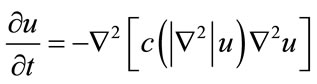
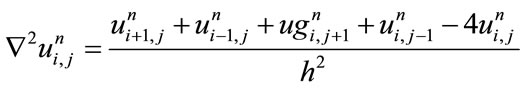
To remove noise, an improved hybrid method [25] is applied to sperm image (R component of RGB color image). This method consists of two stages. The first stage consists of a fourth order partial differential equation (PDE) and the second stage is a relaxed median filter, which processes the output of fourth order PDE. This model enjoys the benefit of both nonlinear fourth order PDE and relaxed median filter. By using a relaxed median filter we can preserve more image details than the standard median filter. This method preserves fine details, sharp corners and thin lines and curved structures to large extent. The L2-curvature gradient flow method of You et al. [33] is used in this model:
 (1)
(1)
where  is the Laplacian of the image u. Since the Laplacian of an image at a pixel is zero if the image is planar in its neighborhood, the PDE attempt to remove noise and preserve edges by approximating an observed image with a piecewise planar image. The desirable diffusion coefficient
  should be such that (1) diffuses more in smooth areas and less around less intensity transitions, so that small variations in image intensity such as noise and unwanted texture are smoothed and edges are preserved. Another objective for the selection of
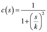
  is to incur backward diffusion around intensity transitions so that edges are sharpened, and to assure forward diffusion in smooth areas for noise removal. The PeronaMalik diffusivity function [34] is used in the implementation as below:
 (2)
(2)
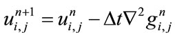
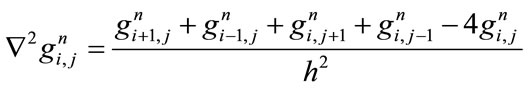
The discrete form of non-linear fourth order PDE described in Eq.1 is as follows:
 (3)
(3)
where
 (4)
(4)
 (5)
(5)
 (6)
(6)
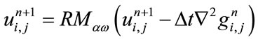
 is the time step size and h is the space grid size. Relaxed median filter [35,36] is used in combination with Eq.1 to remove large spike noises. The proposed hybrid method by Rajan et al. [25] is defined as follows:
 (7)
(7)
where RM is the relaxed median filter with lower bound  and upper bound
 . If
. If  is the output of a relaxed median filter, then
  can be written as
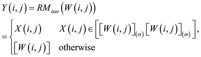 (8)
(8)
where  is the median value of then samples inside the window
 . The sliding window
  is
is
 (9)
(9)
to be the window located at position i. The lower bound and upper bounds for relaxed median used in the experiments are 3 and 5 respectively. By using a relaxed median filter we can preserve more image details than the standard median filter. This method preserves fine details, sharp corners and thin lines and curved structures to large extent. Then, a simple threshold is applied to build a primary mask,  , which contains sperm’s Acrosome, Nucleus and Mid-piece, and also small objects in seminal plasma. The threshold value is calculated according to
 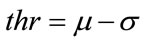 in which
  and
and  are mean and standard deviation of the noise-removed image,
  , respectively. The primary mask,
  is defined as
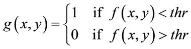 (10)
(10)
The small objects have been eliminated and this mask, containing sperm’s Acrosome, Nucleus and Mid-piece is used to build the final mask at the next step. It is reminded that thr is not enough accurate to detect sperm’s Acrosome, Nucleus, Mid-piece areas in all sperm images (especially about the distal points of Mid-piece). So,  has been only used as a primary mask to build the final mask containing all candidate pixels which may belong to the sperm’s head and Mid-piece.
2.2.2. Finding the Best-Fitted Rectangle for Each Region
To build the final mask, the minimum area bounding box of each individual region is computed through the Rotating Calipers method [26,27]. This method is capable of computing the minimum area enclosing rectangle in linear time. To apply Rotating Calipers method, the two dimensional convex hull of all visible points (for each region) is computed using the monotone chain algorithm [37]. This algorithm is linear with respect to the number of input points O(n), assuming that input points are sorted by increasing x and increasing y coordinates. The minimum rectangle enclosing a convex polygon P has at least one side collinear to one edge of P [26], using this property, a brute-force approach would be to construct an enclosing rectangle for each edge of P. This has a complexity of O(n2) since we have to find minima and maxima for each edge separately. The rotating calipers algorithm rotates two sets of parallel lines (calipers) around the polygon and incrementally updates the extreme values, thus requiring only linear time to find the optimal bounding rectangle. Figure 1 [38] illustrates one step of this algorithm: The support lines are rotated (clock-wise) until a line coincides with an edge of P. If the area of the new bounding rectangle is less than the stored minimum area rectangle, this bounding rectangle becomes the new minimum. This procedure is repeated until the accumulated rotation angle is greater than 90 degrees.
Figure 2 shows the obtained results for each step

Figure 1. Rotating calipers.

Figure 2. Result of applying an improved hybrid method and Rotating Calipers algorithm to a typical sperm image: (a) The original R component of RGB color image; (b) Noise removed image; (c) Selected objects after applying threshold; (d) Primary mask without small objects; (e) Final mask which is created using Rotating Calipers method; (f) Sperm image overlaid on its bounding boxes.
when the proposed method is applied to a typical sperm image. The proposed method for creating a mask containing sperm’s Acrosome, Nucleus and Mid-piece is summarized as below
• Selection of the R component of RGB color image.
• Removing noise from R component using an improved hybrid method.
• Building a primary mask containing sperm’s Acrosome, Nucleus, Mid-piece, and also small objects in seminal plasma, by applying a simple threshold to the noise removed image.
• Elimination of small objects.
• Finding the best-fitted rectangle for each region using rotating calipers.
2.3. Problem Formulation
Support that X is a n-dimensional random variable and comes from a Gaussian mixture model of M > 1 components. Then the probability density function of the Gaussian mixture model can be repressed as the following:
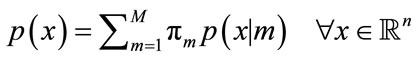 (11)
(11)
where  corresponds to the weight of each component which satisfies
 . For the Gaussian mixtures model, each component density
  is a Gaussian probability density given by
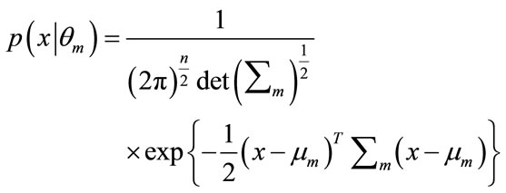 (12)
(12)
where T denotes the transpose operation,  is the mean vector and
  is the covariance matrix which is assumed positive definite. Here we encapsulate these parameters into a parameter vector, writing the parameters of each component as
 , to get
 . Eq.11 can be rewritten as
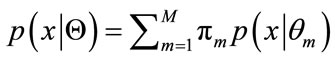 (13)
(13)
If we knew the component from which x came, then it would be simple to determine the parameters . Similarly, if we knew the parameters
 , we could determine the component that would be most likely to have produced x. The difficulty is that we know neither.
2.4. Bayesian Classification
Bayesian Classification is a probabilistic technique of pattern recognition and is based on the principle of Bayes decision theory [39], given in Eq.14 below
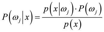 (14)
(14)
where, x is a given feature vector,  denotes a class, or state of nature,
  is the prior probability of class
 ,
,  is prior probability of the feature vector x,
  is aposteriori probability, which a feature vector should be classified as belonging to class
 ,
,  is the conditional probability that a feature vector occurs in a given class
 . For the approach here, the feature x shall consist of one component, intensity of brain pixels. The quantity
  is known as the evidence, and serves only as a scale factor, such that the quantity in Eq.14 is indeed a true probability, with values between zero and one. So, the maximum a posteriori (MAP) estimate of Eq.14 is used as below
 (15)
(15)
According to Bayesian theory [40], the feature vector x is classified to  of which the aposteriori probability given x is the largest between the classes.
 (16)
(16)
Bayes decision rule is optimal in the sense of minimization of the probability of error. It is quite obvious that such an Ideal Bayesian solution can be used only if distributions , and the apriori probabilitles
are known. In the context of classification of brain tissue, the probability models are not known, and therefore, must be approximated. The performance of the Bayesian classifier is directly related to how well these distributions can be modeled.
2.5. Segmentation of Sperm’s Acrosome, Nucleus and Mid-Piece
Sperm’s Acrosome, Nucleus and Mid-piece are segmented using a fully automatic method which is based on entropy based EM algorithm and Markov random field model [29]. This method estimates a gaussian mixture model with three kernels as Background, Nucleus and a class of Acrosome and Mid-piece. To estimate this model, an automatic Entropy based EM algorithm [28] was used to find the best estimated Model. Then, Markov random field (MRF) model and EM algorithm were utilized to obtain and upgrade the class conditional probability density function and the apriori probability of each class. After estimation of Model parameters and apriori probability, samples in bounding boxes were classified using Bayesian classification.
Based on the explanations mentioned above, the block diagram of our method for segmentation of sperm’s Acrosome, Nucleus and Mid-piece is shown in Figure 3,
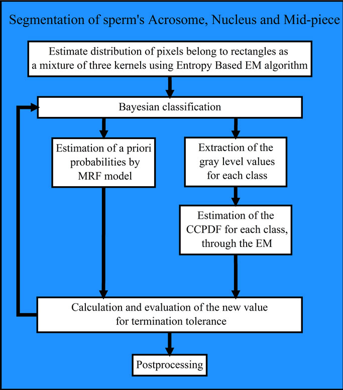
Figure 3. Block diagram of the proposed approach for fully automatic segmentation of sperm’s Acrosome, Nucleus and Midpiece.
and is summarized below 1) Smoothing the R component of RGB color image using a Gaussian filter.
2) Selection of pixels inside the bounding boxes as input samples.
3) Estimation of input samples distribution using Entropy based EM algorithm and Markov Random Field Model [29] with three kernels as Background, Nucleus and a class of Acrosome and Mid-piece.
4) Bayesian classification of the input image (only pixels inside the bounding boxes) using the obtained Gaussian Mixture Model.
5) Postprocessing: Acrosome and Mid-piece are classified into the same class (i.e., two separated areas in one class). These two areas are grouped into two separated classes (i.e., Acrosome and Mid-piece) using their positions respect to the Nucleus and bounding box corners. At first, the distance between each corner of bounding box and center of Nucleus is computed. Then, the corner whose value is less than others is considered as origin. Acrosome is the region whose distance from origin is less than Mid-piece (other region).
2.6. Simulation Results: Segmentation of Sperm’s Acrosome, Nucleus and Mid-Piece
Figure 4 shows the results of the proposed algorithm for a typical sperm image, including estimated distribution obtained through the Entropy based EM algorithm and MRF model overlaid on distribution of the samples (inside the bounding boxes). In Figure 5, results of applying the proposed algorithm to other sperm images have been shown.
2.7. Identification of Sperm’s Tail
After localized segmentation of sperm’s Acrosome, Nucleus and Mid-piece, the pixel at the distal point of sperm’s Mid-piece is considered as an initial point. The method [32] uses a structural similarity index [30] and Rényi entropy [31] in an iterative scheme to estimate sperm’s tail with some points which are placed on the sperm’s tail, accurately. These estimated points can be used to analyze characteristics of sperm’s tail such as length, shape, and etc.
Let X be a digital image of size (M × N) which consists of a sperm, and A be a pixel on the sperm’s tail which is considered as an initial point (point A). Figure 6(a) shows a typical sperm image, a section of sperm’s tail is zoomed in and shown in Figure 6(b). Suppose the bright green pixel is point A, to find the next pixel which is on the sperm’s tail and has the highest structural similarity index (SSIM) with respect to point A, we have used two widows (w1: p × p) and w2: k × k, k < p).
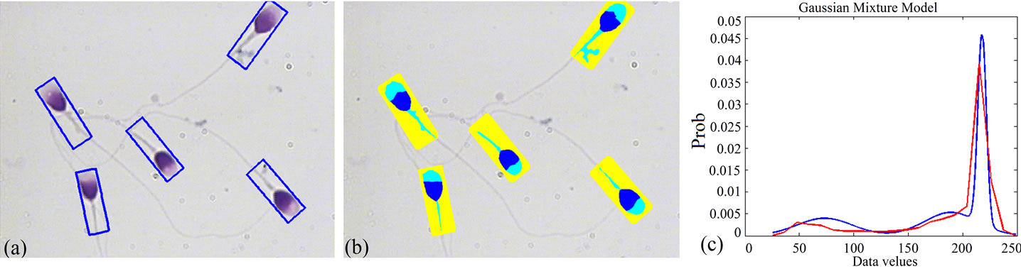
Figure 4. Result of applying the proposed algorithm to a typical sperm image: (a) Bounding boxes containing sperm’s Acrosome, Nucleus and Mid-piece; (b) Result of fully automatic segmentation; (c) Distribution of the samples (red), overlaid on its final estimation (blue). (For interpretation of the references to color in this figure, the reader is referred to the web version of this article).
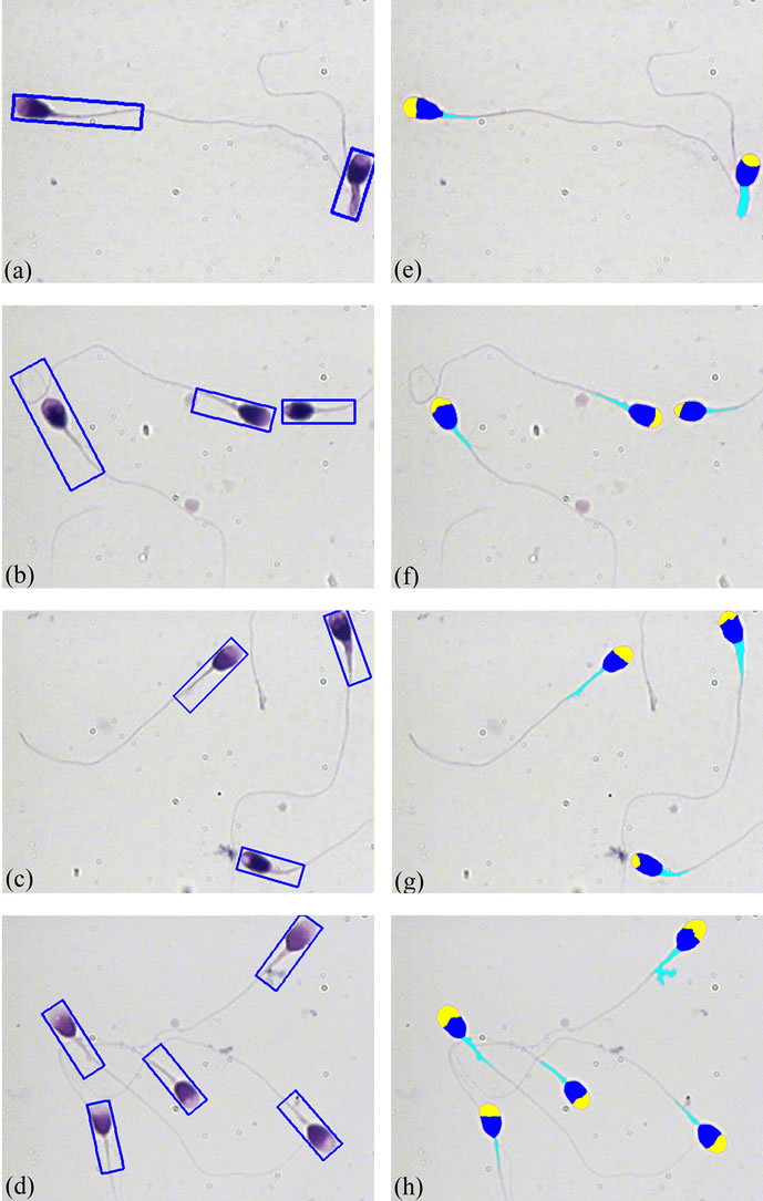
Figure 5. Result of applying the proposed method to three sperm images: (a)-(d) Bounding boxes in the original RGB color images; (e)-(h) Results of fully automatic segmentation. (For interpretation of the references to color in this figure, the reader is referred to the web version of this article).
w1 is centered at point A and is applied to limit A’s neighborhood. Figure 6(b) shows w1 in pink. w2 is a sliding window which moves over the boundaries of w1 and computes the local structural similarity (SSIM) index for each pixel with respect to point A. Figure 6(c) shows pixels which are placed on the boundaries of w1 in deep pink, also different positions of the sliding window (w2) which moves over the boundaries of w1 is shown in blue. So, the SSIM index is calculated within the sliding window (w2) for all pixels which are placed on the boundaries of w1 to find the pixel with the highest SSIM index. SSIM index for all pixels are calculated and scaled ([0,255]), these values are shown in Figure 6(d). The pixel (Point B) which has the highest SSIM index and pixel A are shown in Figure 6(e). If we do the same algorithm for new selected pixel (B), it is possible to select previous pixel (A) as a new pixel. So, before running the new iteration for the new selected pixel, a neighborhood of previous pixel is changed to a different value (say zero). This process is done through another window (w3: l × l, k < l < p). Figure 6(f) shows this process.
This algorithm is implemented in an iterative scheme, and for every new selected pixel, local entropy is computed to detect if we have reached the end of the tail or not.
In this way, for every new selected pixel, the local en tropy is estimated. To estimate the local entropy for every new selected pixel, a window with odd size (w4, h × h) is centered at that pixel, then for every pixel which is placed inside the window, only Red and Green components are extracted as a two dimensional feature. The local entropy is estimated by estimation of the entropy of these samples. Figure 7 shows variations of the local
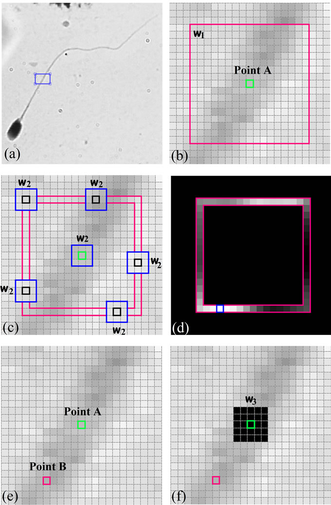
Figure 6. Use of SSIM index to find pixels with the most similarity: (a) A typical sperm image (Red component of RGB color image); (b) The initial pixel (bright green) and w1 (deep pink); (c) w2, sliding window (blue), which computes SSIM for each pixels over the boundaries of w1 and the initial pixel; (d) SSIM values over the boundaries of w1; (e) The new selected pixel with the highest SSIM index (deep pink) and the initial pixel (bright green); (f) A neighborhood of the initial pixel is set to zero. (For interpretation of the references to color in this figure, the reader is referred to the web version of this article).
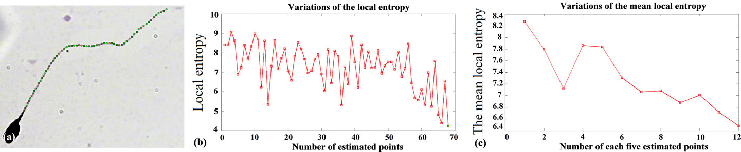
Figure 7. Result of applying the proposed algorithm to the sperm’s image: (a) Estimated points, as the result of proposed method; (b) Variations of the local entropy for estimated points on the sperm’s tail; (c) The mean value of local entropies, for every five selected pixels.
entropy on the sperm’s tail. As it is seen, by reaching the end of sperm’s tail, the local entropy decreases. So, by finding a fitted threshold we would be able to stop the algorithm at the end of sperm’s tail, automatically. We have experimentally observed that a two dimensional feature which contains Red and Green components, gives more strict threshold in comparison with other features.
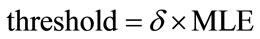
For a fitted threshold, if the estimated value is greater than the threshold, it means that the selected pixel is placed on the sperm’s tail. In other words, the local entropy is considered as a criterion which shows that if we are on the sperm’s tail or not. Finding such a threshold for all sperms is a challenging task. To tackle this problem, the localized thresholding is used. For every five new selected pixels, the local entropy is computed. Then, the mean value of local entropies is considered to compare with a threshold which is called window-threshold. The window-threshold is a fitted threshold for all sperms, and is used to find out if we are close to the distal points of sperm’s tail or not. So, for every five new selected pixels, local entropies are computed and mean value is compared with the window-threshold, if it is greater than the window-threshold, it means that we are not close to the distal points of sperm’s tail and the algorithm must be continued to find five new estimated points in the next five iterations. Otherwise, if the mean value is less than window-threshold, we are close to the distal points and the algorithm must be continued by individual thresholding for every new selected pixel to stop the algorithm in the next five iterations which will be the last ones. Means that from this moment onwards, the algorithm will find at most five new estimated points, in next iterations. Because, by checking the window-threshold, we have found out that we are close to the distal points of sperm’s tail. For individual thrsholding, the minimum local entropy (MLE) of five previous selected pixels is used for thresholding as below
 (17)
(17)
 has been experimentally set to 0.9 for the best result.
The algorithm for detection of sperm’s tail includes two major modules:
• Selecting an initial pixel (A) which is placed at the end of mid-piece, and finding the pixel (B) with the highest SSIM index respect to that. To compute and compare the structural similarity (SSIM) index, only the Red component of the RGB color image is considered as a separate image and is used to perform this module.
• Verifying if the selected pixel (B) is on the sperm’s tail or not, this procedure is based on the local entropy estimation. To evaluate the local entropy, only the Red and Green components of RGB color image are used as a two dimensional feature.
The steps of proposed method are described in detail as below:
1) Setting pixels on the sperm’s head and mid-piece to a different value (say zero).
2) Smoothing the input image using an average filter.
3) Selecting the distal point of sperm’s Mid-piece as the initial point, pixel (A), and setting the Counter to one.
4) Centering the window w1 at pixel A.
5) Moving a sliding window (w2) over w1’s boundaries and compute SSIM index, locally, through Eq.12, for each pixel over the boundaries of w1 and pixel A.
6) Finding the pixel with the largest amount of SSIM Index (B).
7) Estimation of the local Entropy at pixel B.
8) Setting pixels around the new selected pixel (B) to a different value (say zero), through the window w3.
9) Replacing the initial pixel (A) with the new selected pixel (B).
10) Checking the Counter: if the Counter is equal to five, go to the next step, otherwise increase the Counter by one and go to the Step 4.
11) Checking the localized thresholding: compute the mean value of the local entropies of the last five selected pixels. If it is greater than the window-threshold, set the Counter to one and go to the Step 4, otherwise find the minimum local entropy (MLE) of the last five selected pixels and go to the next step.
12) Repeating Steps 4-9 to find the new estimated pixel.
13) Comparing the local entropy of the new selected pixel with the threshold (Eq.17). If it is greater than the threshold, go to the step 12 to find a new pixel on the sperm’s tail, otherwise stop the algorithm.
2.8. Simulation Results: Identification and Discrimination of Sperm’s Tail
The results of the proposed method, for different sperms are shown in Figure 8. Figures 8(a)-(d) show the original sperm images. The proposed method is applied to sperm images, and the estimated points are shown in Figures 8(e)-(h). As it is seen, the estimated points are exactly located on the sperm’s tail. Figures 8(i)-(l) show how the estimated local entropy changes with the position of estimated points on the sperm’s tail. The last points in each tail have the lowest value of local entropy in comparison with the other points, these values are less than the threshold, and the algorithm was stopped because of these points.
3. EVALUATION
The algorithms were tested with a 100 slides database with multiple spermatozoa (including 283 sperms). The first stage tested was the “detection and extraction of individual spermatozoon” with the entire image database. In this research, criteria Accuracy (Ac), Sensitivity (Se) and Specificity (Sp) are used for evaluation.
 (18)
(18)
 (19)
(19)
 (20)
(20)
In these equations, TP is the number of true positive, FP is the number of false, TN is the number of true negative, and FN is the number of false negative. The evaluation is summarized in Table 1.
Also the, Accuracy of sperm’s head, Acrosome, Nucleus and Mid-piece are computed 94.3%, 92.4%, 95.1% and 90.2%, respectively. For all sperms in database, sperm’s tail length is computed manually and compared with the estimated value through the estimated points. Success rate [32] is defined below
 (21)
(21)
and computed for all sperms. The overall Success Rate of this approach is 97.6%.
4. DISCUSSION
In this paper a new approach, for fully automatic identification and discrimination of sperm’s Acrosome, Nucleus, Mid-piece and tail in microscopic images of stained human semen smear that requires no training and atlas, is proposed. The proposed method includes two major modules. At first, to increase the detection rate and speed, a localized mask containing sperm’s Acrosome, Nucleus and Mid-piece is built through the minimum area bounding boxes. This procedure is done using an improved hybrid method and the Rotating Calipers algorithm. Pixels inside the bounding boxes are considered as samples. Distribution function of samples is estimated by
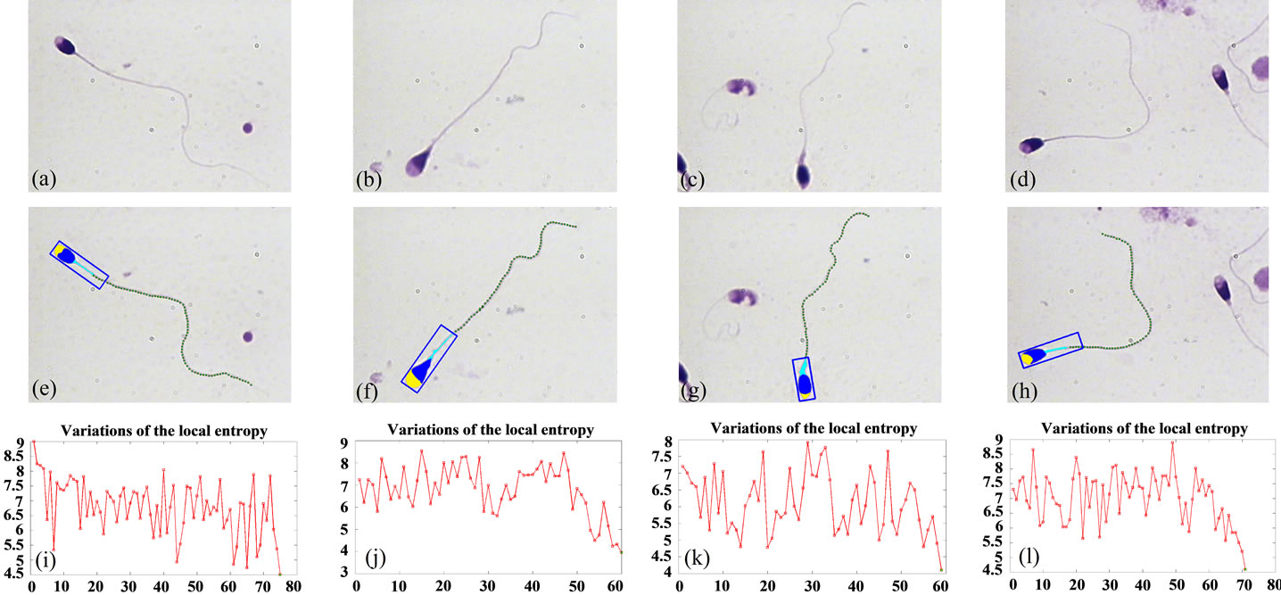
Figure 8. Result of applying the proposed algorithm to different sperms images: (a)-(d) Original sperm images; (e)-(h) Estimated points, as the result of the proposed method; (i)-(l) Use of local entropy changes as a measure for identification of end of tails.

Table 1. Evaluation results for detection and extraction of individual spermatozoon.
a mixture of a large number of normal terms by AMM. Then, the mixture terms are categorized into three classes, as the CCPDFs and the apriori probabilities of the classes. In the next steps, apriori probabilities of the classes as well as parameters of the classes (i.e., means and variances) are attained and updated, utilizing MRF model and AMM, respectively, and without any need for training samples. After segmentation of sperm’s Acrosome, Nucleus and Mid-piece, the distal point of midpiece is considered as an initial point. Knowing that a pixel is located on the sperm’s tail (such as the distal point of mid-piece), to find a new pixel on the sperm’s tail, SSIM index is computed and checked, locally. To automatically stop the algorithm at the end of sperm’s tail, local entropy is selected and estimated as a feature. These estimated points could be used to verify the morphological characteristics of sperm’s tail such as length, shape and etc. The accuracy of proposed method depends on the parameters of Structural Similarity (SSIM) index (i.e., α, β and γ) which adjust the relative importance of the Luminance, contrast and Structure comparison components. Figure 9(a) shows a typical sperm image, a section of sperm’s tail is zoomed in and shown in Figure 9(b). The boundary of sperm’s tail is segmented, manually, and is shown in black. Also, a pixel on the sperm’s tail is selected as an initial point and shown in deep pink (point A). Figure 9(c) shows pixels which have been selected to find the pixel with the highest SSIM index respect to point A (according to the proposed method). To understand the relative importance of comparison components, SSIM index is computed individually for each comparison component and is shown in Figures 9(d)-(f):
• SSIM index based on Luminance comparison component (α = 1, β = 0 and γ = 0).
• SSIM index based on contrast comparison component (α = 0, β = 1 and γ = 0).
• SSIM index based on Structure comparison component (α = 0, β = 0 and γ = 1).
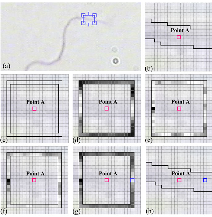
Figure 9. Relative importance of comparison components: (a) A typical sperm image; (b) A section of sperm’s tail containing it’s manual segmentation is zoomed in, and a pixel on the sperm’s tail is selected as an initial point (deep pink, point A); (c) Point A and it’s limited neighborhood (according to the proposed method); (d) SSIM values based on Luminance comparison component (α = 1, β = 0 and γ = 0); (e) SSIM values based on contrast comparison component (α = 0, β = 1 and γ = 0); (f) SSIM values based on Structure comparison component (α = 0, β = 0 and γ = 1); (g) SSIM values with α = 0.1, β = 0.5 and γ = 0.9, the new selected pixel with the highest SSIM index is shown in blue; (h) Manual segmentation of sperm’s tail, initial pixel (point A) and the new selected pixel. (For interpretation of the references to color in this figure, the reader is referred to the web version of this article).
As it is seen, pixels which are placed on the sperm’s tail have higher Luminance comparison components in comparison with others. Also, in addition to pixels which are placed on the sperm’s tail, there are some other pixels over the boundary which have higher values for contrast and Structure comparison components. So, Luminance comparison component has the most relative importance.
As mentioned before, structural similarity index satisfies the Boundedness condition (SSIM < 1), that’s way α, β and γ have been experimentally set to 0.1, 0.5 and 0.9 for the best result.
One of the important advantages of the proposed method is the ability to detect sperm’s tail in the lowcontrast sections. Also, the execution time of implemented algorithm is too low. Our proposed approach is evaluated via Accuracy, Sensitivity, Specificity and Success Rate in a data set of microscopic images of stained human semen smear.
Some other methods have been developed to analyze human sperm morphology, the primary steps of all these
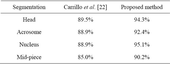
Table 2. Accuracy (Ac) values for the proposed method and Carrillo et al. [22].
methods is sperm segmentation and discrimination. Sánchez et al. [4,15] and Nowshiravan et al. [19] proposed methods based on morphological operators and thresholding to segment sperm’s head, Because the Acrosome and the Mid-piece have similar characteristics (intensity level, texture) the segmentation with traditional techniques (thresholding, region growing) does not give good results [19,20]. To tackle this problem, Carrillo et al. [22, 23] presented an approach called nth-fusion for segmentation of sperm’s Acrosome, Nucleus and Mid-piece in a computer aided tool for the objective analysis of human sperm morphology, commonly known as Automated Sperm Morphology Analyzer (ASMA). After enclosing individual sperms (head and Mid-piece) using bounding boxes, they used nth-fusion method which was based on nth-level thresholding of an image followed by intersection with n special masks. In order to obtain the desired segmentation results, aprior objects morphological model, which was based on the information fusion technique in a feature level was used. For each segmented sperm in image, they had to run the algorithm to detect sperm’s parts. It is reminded that Carrillo et al. [22] used manual segmentation for evaluation of their methods. We, too, used manual segmentation for evaluation. They used similar methods of evaluation. Therefore comparison of our method with this method is reasonable. This comparison is done in Table 2. As it is seen in Table 2, the proposed method in this paper improves the accuracy of segmentations. The drawback of the proposed method for detection and discrimination of sperm’s tail is that objects which are placed on the sperm’s tail, affect the performance of the proposed method. So, In future investigations we intend to use various geometric features to increase accuracy values.
![]()
![]()
REFERENCES
- Domar, A.D., Broome, A., Zuttermeister P.C., Seibel, M. and Friedman, R. (1992) The prevalence and predictability of depression in infertile women. Fertility and Sterility, 58, 1158-1163.
- World Health Organization (1999) WHO laboratory manual for examination of human semen and sperm cervical mucus interaction. 4th Edition, Cambridge University Press, Cambridge.
- Katz, D.F., Overstreet, J.W., Samuels, S. J., Niswander, P.W., Bloom, T. D. and Lewis, E.L. (1985) Morphometric analysis of spermatozoa in the assessment of human male fertility. Journal of Andrology, 7, 203-210.
- Sánchez L., Petkov, N. and Alegre, E. (2006) Statistical approach to boar semen evaluation using intracellular intensity distribution of head images. Cellular and Molecular Biology, 52, 38-43. doi:10.1170/T736
- Gravance, C.G., Garner, D.L., Pitt, C., Vishwanath, R., Sax-Gravance, S.K. and Casey, P.J. (1999) Replicate and technician variation associated with computer aided bull sperm head morphometry analysis (ASMA). International Journal of Andrology, 22, 77-82. doi:10.1046/j.1365-2605.1999.00148.x
- Hirai, M., Boersma, A., Hoeflich, A., Wolf, E., Foll, J., Aumuller, T. and Braun, J. (2001) Objectively measured sperm motility and sperm head morphometry in boars (Sus scrofa): Relation to fertility and seminal plasma growth factors. Journal of Andrology, 22, 104-110.
- Wijchman, J., Wolf, B.D., Graafe, R. and Arts, E. (2001) Variation in semen parameters derived from computeraided semen analysis, within donors and between donors. Journal of Andrology, 22, 773-780.
- Quintero-Moreno, A., Rigaub, T. and Rodrguez-Gil, J.E. (2001) Regression analyses and motile sperm subpopulation structure study as improving tools in boar semen quality analysis. Theriogenology, 61, 673-690. doi:10.1016/S0093-691X(03)00248-6
- Rijsselaere, T., Soom, A.V., Hoflack, G., Maes, D. and de Kruif, A. (2004) Automated sperm morphometry and morphology analysis of canine semen by the HamiltonThorne analyser. Theriogenology, 62, 1292-1306. doi:10.1016/j.theriogenology.2004.01.005
- Verstegen, J., Iguer-Ouada, M. and Onclin, K. (2001) Computer assisted semen analyzers in andrology research and veterinary practice. Theriogenology, 57, 149-179. doi:10.1016/S0093-691X(01)00664-1
- Beletti, M., Costa, L. and Viana, M. (2005) A compareson of morphometric characteristics of sperm from fertile bos taurus and bos indicus bulls in Brazil. Animal Reproduction Science, 85, 105-116. doi:10.1016/j.anireprosci.2004.04.019
- Garrett, C. and Baker, H. (1995) A new fully automated system for the morphometric analysis of human sperm heads. Fertility and Sterility, 63, 1306-1317.
- Linneberg, C., Salamon, P., Svarer, C. and Hansen, L. (1994) Towards semen quality assessment using neural networks. Proceedings of IEEE Neural Networks for Signal Processing IV, Ermioni, 6-8 September 1994, 509- 517.
- Ostermeier, G., Sargeant, G., Yandell, T. and Parrish, J. (2001) Measurement of bovine sperm nuclear shape using Fourier harmonic amplitudes. Journal of Andrology, 22, 584-594.
- Sánchez, L., Petkov, N. and Alegre, E. (2005) Statistical approach to boar semen head classification based on intracellular intensity distribution. In: Gagalowicz, A. and Philips, W. Eds., Proceedings of the International Conference on Computer Analysis of Images and Patterns, Lecture Notes in Computer Science, Springer, Berlin, 88- 95.
- Otsu, N. (1979) A threshold selection method from graylevel histograms. IEEE Transactions on Systems, Man and Cybernetics, 9, 62-66. doi:10.1109/TSMC.1979.4310076
- Biehl, W.M., Pasma, P., Pijl, M., Sánchez, L. and Petkov, N. (2006) Classification of boar sperm head images using learning vector quantization. In: Verleysen, M., Ed., Proceedings of the European Symposium on Artificial Neural Networks (ESANN), Brugge, 26-28 April 2006, 545-550.
- Alegre, E., Biehl, M., Petkov, N. and Sánchez, L. (2008) Automatic classification of the acrosome status of boar spermatozoa using digital image processing and LVQ. Computers in Biology and Medicine, 38, 461-468. doi:10.1016/j.compbiomed.2008.01.005
- Nowshiravan Rahatabad, F., Moradi, M.H. and Nafisi, V.R. (2005) A multi steps algorithm for sperm segmentation in microscopic image. Proceedings of the World Academy of Science, Engineering and Technology, 12, 43-45.
- Nafisi, V.R., Moradi, M.H. and Nasr-Esfahani, M.H. (2005) Sperm identification using elliptic model and tail detection. Proceedings of the World Academy of Science, Engineering and Technology, 6, 205-208.
- Park, K., Yi, W. and Paick, J. (1997) Segmentation of sperms using the strategic Hough transform. Annals of Biomedical Engineering, 25, 294-302. doi:10.1007/BF02648044
- Carrillo, H., Villarreal, J., Sotaquira, M., Goelkel, M. and Gutierrez, R. (2007) A computer aided tool for the assessment of human sperm morphology. Proceedings of the 7th IEEE International Conference on Bioinformatics and Bioengineering (BIBE), Boston, 14-17 October 2007, 1152-1157. doi:10.1109/BIBE.2007.4375706
- Carrillo, H., Villarreal, J., Sotaquira, M., Goelkel, M. and Gutierrez, R. (2005) Spermatozoon segmentation towards an objective analysis of human sperm morphology. Proceedings of the 5th International Symposium on image and Signal Processing and Analysis, Zagreb, 15-17 September 2005, 522-527.
- Abbiramy V.S. and Shanthi, V. (2010) Spermatozoa segmentation and morphological parameter analysis based detection of teratozoospermia. International Journal of Computer Applications, 3, 19-23. doi:10.5120/743-1050
- Rajan, J., Kannan, K. and Kaimal, M.R. (2008) An improved hybrid model for molecular image denoising. Journal of Mathematical Imaging and Vision, 31, 73-79. doi:10.1007/s10851-008-0067-4
- Pirzadeh, H. (1999) Computational geometry with the rotating calipers. Master’s Thesis, School of Computer Science, McGill University, Montreal.
- Toussaint, G.T. (1983) Solving geometric problems with the rotating calipers. Proceedings of IEEE MELECON83, Athens, 24-26 May 1983.
- Benavent, A.P., Ruiz, F.E. and Sáez, J.M. (2009) Learning gaussian mixture models with entropy-based criteria. IEEE Transactions on Neural Networks, 20, 1756-1771. doi:10.1109/TNN.2009.2030190
- Bijar, A., Mohamad Khanloo, M., Benavent, A.P. and Khayati, R. (2011) Segmentation of MS lesions using en-tropy-based EM algorithm and Markov random fields. Journal of Biomedical Science and Engineering (JBISE), 4, 552-561. doi:10.4236/jbise.2011.48071
- Wang, Z., Bovik, A.C., Sheikh, H.R. and Simoncelli, E.P. (2004) Image quality assessment: From error measurement to structural similarity. IEEE Transaction on Image Processing, 13, 1-14. doi:10.1109/TIP.2003.819861
- Rényi, A. (1961) On measures of entropy and information. Proceedings of the 4th Berkeley Symposium on Mathematical Statistics and Probability, Berkeley, 20 June-30 July 1960, 547-561.
- Bijar, A. and Mikaeili, M. (2011) Sperm’s tail identification and discrimination in microscopic images of stained human semen smear. Proceeding of the 7th International Symposium on Image and Signal Processing and Analysis (ISPA), Croatia, 4-6 September 2011, 709-714.
- You, Y.L. and Kaveh, M. (2000) Fourth-order partial differential equations for noise removal. IIEEE Transactions on Image Processing, 9, 1723-1730. doi:10.1109/83.869184
- Perona, P. and Malik, J. (1988) Scale-space and edge detection using anisotropic diffusion. IEEE Transactions on Pattern Analysis and Machine Intelligence, 12, 629- 639. doi:10.1109/34.56205
- Hamza, A.B., Escamilla, P.L., Aroza, J.M. and Roldan, R. (1999) Removing noise and preserving details with relaxed median filters. Journal of Mathematical Imaging and Vision, 11, 161-177. doi:10.1023/A:1008395514426
- Hamza, A.B. and Krim, H. (2001) Image denoising: A nonlinear robust statistical approach. IEEE Transactions on Signal Processing, 49, 3045-3054. doi:10.1109/78.969512
- Andrew, A. (1997) Another efficient algorithm for convex hulls in two dimensions. Information Processing Letters, 9, 216-219. doi:10.1016/0020-0190(79)90072-3
- Brabec, S., Annen, T. and Seidel, H.P. (2002) Practical shadow mapping. Journal of Graphics, GPU, and Game Tools, 7, 9-18.
- Duda, R.O., Hart, P.E. and Stork, D.G. (2001) Pattern classification. 2nd Edition, Wiley, New York.
- Bernardo, J.M. and Smith, A.F.M. (1994) Bayesian theory. Wiley, New York. doi:10.1002/9780470316870