Intelligent Information Management
Vol.2 No.6(2010), Article ID:2029,6 pages DOI:10.4236/iim.2010.26046
The Line Clipping Algorithm Basing on Affine Transformation
College of Math and Computer Science, Guangxi University for Nationalities, Nanning, China
E-mail: hwjart@126.com
Received March 20, 2010; revised April 25, 2010; accepted May 27, 2010
Keywords: Computer Graphics, Line Clipping, Algorithm, Affine Transformation
Abstract
A new algorithm for clipping line segments by a rectangular window on rectangular coordinate system is presented in this paper. The algorithm is very different to the other line clipping algorithms. For the line segments that cannot be identified as completely inside or outside the window by simple testings, this algorithm applies affine transformations (the shearing transformations) to the line segments and the window, and changes the slopes of the line segments and the shape of the window. Thus, it is clear for the line segment to be outside or inside of the window. If the line segments intersect the window, the algorithm immediately (no solving equations) gets the intersection points. Having applied the inverse transformations to the intersection points, the algorithm has the final results. The algorithm is successful to avoid the complex classifications and computations. Besides, the algorithm is effective to simplify the processes of finding the intersection points. Comparing to some classical algorithms, the algorithm of this paper is faster for clipping line segments and more efficient for calculations.
1. Introduction and Previous Work
In computer graphics, line clipping is a basic and important operation, and has many applications. For example, extracting part of a defined scene for viewing must take line clipping. The region that includes the part of the defined scene is called a clip window. Generally, the window is a rectangle or a general polygon.
The early and classical algorithms of line clipping are Cohen-Sutherland Line Clipping algorithm [1], CyrusBeck Line Clipping algorithm [2] and Nicholl-Lee-Nicholl Line Clipping algorithm [3].
Cohen-Sutherland Line Clipping algorithm is one of the oldest and most popular line-clipping procedures. The algorithm uses a rectangle window with a coding scheme to subdivide the two-dimensional space which includes the graph. Then, each endpoint of a line segment of the graph is assigned the code of the sub-region in which it lies. And according to the value of the “&” and “|” which are made by the two codes of the two endpoints of the line segment, the algorithm determines the line segment to be inside of the widow or not. For the simple situations (the line segments are completely inside or outside of the window), the algorithm can quickly get the results. But for the line segments that cannot be identified as completely inside or completely outside the window by the scheme of the algorithm, the algorithm has to make computations and turn the line segments into the “simple situations”. Obviously, if the line segment is outside of the window, the computations are waste.
Later, Cyrus-Becky proposed Cyrus & Beck algorithm. The algorithm treats line in parametric form. The theoretical model of this algorithm is general. However, it is rather inefficient. To clip a line segment which is neither vertical nor horizontal and lies entirely within the window, it will perform 12 additions, 16 subtractions, 20 multiplications and 4 divisions [4]. Besides, for the general case (the line segments will cross all the boundaries of the window), the algorithm first makes computations and find the parameters of the intersection points. Then, according to the signs of the denominators of the parameters and the values of the parameters, the algorithm determines which parts of the line segments are inside the window. Clearly, if the line segment is outside of the window, the computations are useless.
In [3], Nicholl-Lee-Nicholl Line Clipping algorithm makes four rays which pass an endpoint of the line segment and four vertexes of the window, and creates three regions by the four rays. Then, the algorithm determines which region that the line segment lies in, and determines finding the intersections or rejecting the line segment. Before finding the intersection points of the line segment and the window, the algorithm first determines the position of the first endpoint of the line segment for the nine possible regions relative to the clipping window. If the point is not in the one of the three especial regions, the algorithm has got to transform the point to the one of the three especial regions. To find the region in which the other endpoint of the line segment lies, the algorithm has got to compare the slope of the line segment to the slopes of the four rays. So, for the algorithm, finding the intersection points are efficient, but finding the positions of the two endpoints of the line segment are more complicated than Cohen-Sutherland Line Clipping algorithm.
Independently, You-dong Liang, Brian A.Barsky, Mel Slater offered a more faster algorithm [5,6]. This algorithm is based on a parametric representation of the line segment. The algorithm is somewhat complicated and inefficient. To clip a line segment which is neither vertical nor horizontal, it will perform 16 comparisons, 7 subtractions, and 4 divisions.
In [7], Vaclv Skala proposed a line clipping algorithm for convex polygon window. The algorithm uses the binary search to find the intersections in the clipping window. The complexity is O (lg N). But for the rectangle window, the algorithm does not have obvious advantage in comparison with the Cyrus-Beck algorithm.
In [8], the authors proposed the Optimal Tree algorithm. Based on the regions (there are nine regions subdivided by the four boundaries of the window) that the endpoints of the line segment lies in, the authors proposed five types of “Partition-Pairs”: the “window-side or side-window” (including 8 cases), the “window-corner or corner-window” (including 16 cases), the “side-side” (including 20 cases), the “side-corner or corner-side” (including 16 cases) and the “corner-corner” (including 4 cases). There are 64 cases in the five types of “Partition-Pairs” and the optimal tree includes these 64 cases. The algorithm performed uniformly faster than all above algorithms. But the algorithm is too complicated.
In [9], the author proposed an algorithm based on homogeneous coordinates. In the algorithm, the author assumes a rectangular window P and a line p given as F(x) = ax + by + c = 0. The line p subdivides the space into two half-spaces as F(x) < 0 and F(x) > = 0. According to the locations of all the vertexes of the window to the line, the author makes out 16 possible cases and makes a table storing the cases. To clipping a line, the algorithm makes the calculations and determines the locations of all the vertexes of the window to the line. Having compared the locations with the cases in the table, the algorithm determines which edges of the window intersect the line and finds the intersection points by the cross products of their homogeneous coordinates. The algorithm is inefficient. To clip a line segment which will cross the window, the algorithm first codes the two endpoints of the line segment, and makes 4 comparisons and 2 cross products (taking 12 multiplications). If turning the intersection points (xi, yi, w) into (xi/w, yi/w), the algorithm still makes 4 divisions. So, in Euclidean space the computational complexity of the algorithm is more than CohenSutherland algorithm.
In this paper, a new line clipping algorithm for a rectangle clip window will be given. Comparing those algorithms above, this algorithm makes the speed of line clipping faster and makes the calculations more efficient.
2. Theorems
2.1. Theorem 1
In a plane, the necessary and sufficient conditions for two line segments without any points of intersection are that there are no any points of intersection of the two line segments after applying an affine transformation to the two line segments.
Proof. We suppose that there are two line segments  (the endpoints are
  and
and ) and
) and  (the endpoints are
  and
and  ) in a plane, and

 =
= . Also, we suppose that there is a affine transformation T, and we apply the affine transformation T to the two line segments
  and
and :
:
T( ) =
) =  (the endpoints are
  and
and )T(
)T( ) =
) =  (the endpoints are
  and
and ).
).
2.1.1. The Sufficient Condition (Proof by Contradiction)
If 

 = A'(A'
 ), we apply the
  (
( exist because T is an affine transformation) to
 and
and , and have
  =
= ,
,  =
= . The
. The  is still an affine transformation. According to the properties of affine transformation, we get the conclusion: Straight line
 straight line

 . So, we set the straight line
 The straight line
 = A (A
 ). Because

 =
= , so the point A
 the extension of the line segment
  or the line segment
 . So
. So
 A/
A/ A > 0 or
  A/
A/ A > 0.
But
 A'/
A'/ A' < 0 and
  A'/
A'/ A' < 0.
Those are contradictory in the properties of affine transformation.
2.1.2. The Necessary Condition
The proof is as same as the proof of the sufficient condition.
From the theorem, two important inferences can be derived:
1) On a plane, the necessary and sufficient conditions for two line segments with a point of intersection are that there is a point of intersection of the two line segments after applying an affine transformation to the two line segments.
2) On a plane, the necessary and sufficient conditions for that a line segment is inside of a window (or outside of the window, or across the window) are that the line segment is inside of the window (or outside of the window, or across the window) after applying an affine transformation to the line segment and the window.
2.2. Theorem 2
In a rectangular coordinate system, we suppose that the slope of a straight line a (The endpoints are  and
and ) is 1/c(c
 0) and the straight line b (The endpoints are
  and
and ) is vertical to the axis x (i.e. b
 the axis x). If apply the affine transformation
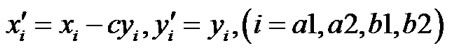
 : x' = x-cy, y' = y; ((x, y) is a point.)
to the line segments a and b, i.e.
a' =  (a) and b' =
  (b).
(b).
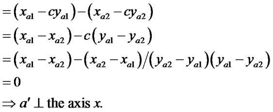
There is a conclusion: The line segment a' the axis x and the slope of b' = –1/c.
Proof.  (a) and
  (b) are
 .
.
1) 
2) 

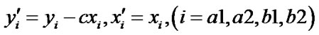
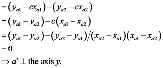
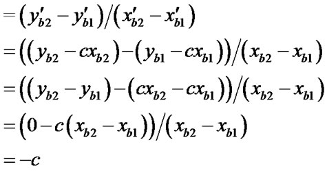
2.3. Theorem 3
In a rectangular coordinate system, we suppose that the slope of a straight line a (The endpoints are  (
( ,
, ) and
) and  (
( ,
, )) is c (c
 0) and the straight line b (The endpoints are
  (
( ,
, ) and
) and  (
( ,
, )) is vertical to the axis y (i.e. b
 the axis y). If apply the affine transformation
 : x' = x, y' = ‑ cx + y; ((x, y) is a point.)
to the line segment a and b, i.e.
a' = (a ) and b' =
 (b)
(b)
There is a conclusion: The line segment a' the axis y and the slope of b'= –c.
Proof.  (a) and
  (b) are
 .
.
1) 
2) 
3. The Basic Idea of the Algorithm
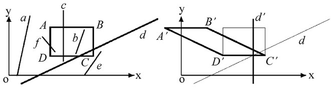
We suppose that there are a rectangular window and some line segments in a rectangular plane coordinate system (see Figure 1).
Four types of the line segments are gotten by classifying the line segments according to the positions against the window.
The first are outside of the rectangular window (see the line segment a in Figure 1(a)).
The second are inside of the rectangular window (see the line segment b in Figure 1(a)).
The third are parallel or vertical to the edges of the rectangular window and intersecting the rectangular window (see the line segment c in Figure 1(a)).
The fourth are the other line segments that do not belong to any types as above (see the line segments d, e, and f in Figure 1(a)).
 (a) (b)
  (c) (d)
In the figure (a) and (d), the vertexes of the window are A ( ,
, ), B (
 ,
, ), C (
 ,
, ) and D (
 ,
, ).
).
In the figure (b), the vertexes of the window are (
( ,
, ),
),  (
( ,
, ),
),  (
( ,
, ) and
) and  (
( ,
, ).
).
In the Figure (c), the vertexes of the window are  (
( ,
, ),
),  (
( ,
, ),
),  (
( ,
, ) and
) and  (
( ,
, ).
).
Figure 1. The process of the clipping. (a) Lines and window; (b) Tx(d) and Tx(w); (c) Ty(d) and Ty(w); (d) The result.
For the first, the second and the third, we process them with subtraction. For the fourth, we apply the affine transformations to the line segments of the fourth and apply the same affine transformations to the window with the theorem 2 and the theorem 3, turning the fourth into the line segments that are vertical or parallel to axis x, and turning the window into a parallelogram that have two edges which are vertical to the line segment (see Figures 1 (b) and (c)). Now, according to theorem 1 ~ theorem 3, we can easily determine the line segment is outside of the window or across the window.
After getting the intersections of the line segment and the window, we apply the inverse transformations of the affine transformations to the intersections, and the line segment clipped by the window is gotten.
4. The Steps of the Algorithm
/*In the step (2), (3), (4) and (5), we process the first, the second, the third and the fourth as above orderly.*/
1) Preparation:
Give a rectangular plane coordinate system xoy;
Give four edges of a rectangular window W:
float ,
,  ,
,  ,
,  , (
, ( <
< ,
, <
< );
);
Give a line segment randomly:
float  (
( ,
, ),
),  (
( ,
, ); int flag: = 0;
float  (
( ,
, ): =
): = (
( ,
, ),
),
 (
( ,
, ): =
): = (
( ,
, );
);
int : = (
: = (


 ) && (


 );
);
int : = (
: = (


 ) && (


 );
);
2) if (( and
and )
)
 ) || ((
 and
and )
)
 ) || ((
 and
and )
)
 ) || ((
 and
and )
)
 ), goto (7);
3) else if ( &&
&& ), goto (6);
4) else if ( =
= ) {
) {
if ( >
> ){ swap(
 ,
, ); swap(
 ,
, );}
);}
if (

 ) and (

 )
)
{ : =
: = ;
; : =
: = ; goto (6);}
else if (

 ) and (

 )
)
{ : =
: = ; goto (6);}
else if (

 ) and (

 )
)
{ : =
: = ; goto (6);}
}
else if ( =
= ) {
) {
if ( >
> ){ swap(
 ,
, ); swap(
 ,
, );}
);}
if (

 ) and (

 )
)
{ : =
: = ;
; : =
: = ; goto (6);}
else if (

 ) and (

 )
)
{ : =
: = ; goto (6);}
else if (

 ) and (

 )
)
{ : =
: = ; goto (6);}
}
5) else{
5.1) c: = ( -
- )/(
)/( -
- );
);
5.2) if ( >
> ) {swap (
 ,
, ); swap(
 ,
, );}
);}
 : =
: = (
( );
); : =
: = (
( ); w':=
  (w);
(w);
/*After getting the affine transformation, the rectangular window become a parallelogram having two edges that parallel to axis x, and the line segment ( ,
, ) is vertical to the axis x. See Figure 1(b).*/
5.3) if (c >0) && ((

 ) || (

 )) goto (7);
/*see Figure 1(b)*/
else if(c < 0) && ((

 ) || (

 )) goto(7); /*refer to the Figure 1(b)*/
else {
if (

 ) and (

 ) {flag++;
if (

 ) and (

 )
) =
= ;
;
 =
= (
( );
); =
= (
( );
);
}
if (

 ) and (

 ) {flag++;
if (

 ) and (

 )
) =
= ;
;
 =
= (
( );
); =
= (
( );
);
}
if (flag = 2) goto (6);
/*“flag = 2” means that the line clipping have been finished.*/
5.4) if ( >
> ){swap(
 ,
, ); swap(
 ,
, );} c: = 1/c;
 : =
: = (
( );
); : =
: = (
( ); w' =
 (w);
(w);
/*After getting the affine transformation, the rectangular window become a parallelogram having two edges that parallel to axis y, and the line segment ( ,
, ) is vertical to the axis y. See Figure 1(c).*/
5.5) if (

 ) and (

 ) {flag++;
if (

 ) and (

 )
) =
= ;
;
 =
= (
( );
); =
= (
( );
);
}
if (![]()

 ) and (

 ) { flag++;
if (

 ) and (

 )
) =
= ;
;
 =
= (
( );
); =
= (
( );
);
}
/*see Figure 1 (c)*/
}
6) Drawing the line ( ,
,  ,
,  ,
, );
);
7) The end;
5. The Calculation Complexity
In the most complex case (the lines belong to the fourth type as above), after using 2 divisions to get the slope and the 1/slope of a line segment, the algorithm uses two steps with 4 multiplications to make the clipping.
First, the algorithm translates the window and places the “bottom edge” on the axis x, and makes the same translation for the line segment. Then, it uses one multiplication to apply an affine transformation to the “top edge” of the window and uses another multiplication to get the intersection of the window and the line segment (see Figure 1(b)).
Second, the algorithm translates the window and places the “left edge” on the axis y, and applies the translation to the line segment. Then, it uses one multiplication to apply an affine transformation to the “right edge” of the window and use another multiplication to get the intersection of the window and the line segment (see Figure 1(c)).
So, the algorithm at most uses 2 divisions and 4 multiplications to finish the clipping for a line segment (See table 1).
Here, we list the calculation complexities of the algorithm and other algorithms in table 1 for comparing. Where “C-S algorithm”, “C-B algorithm”, “N-L-N algorithm”, “L-B algorithm”, “VS algorithm” and “L-B-2 algorithm” indicate that the Cohen-Sutherland Algorithm [1], the Cyrus-Beck Algorithm [2], the Nicholl-LeeNicholl Algorithm [3], the Liang-Barsky-Slater Algorithm [5,10], the O(lg N) Line Clipping Algorithm in  [7] and the Optimal Tree Algorithm for Line Clipping [8] orderly.
6. Results and Discussion
The algorithm in this paper has been realized with a computer in C language with TC system. It is successful for the algorithm to clip the random line segments (see Figure 1(a)). We take the special situation like line segment d in Figure 1 for a sample to perform the process of the clipping and to make comparisons. The comparisons between the algorithm in this paper and Cohen-Sutherland algorithm have been list in table 2. In table 2, the first row give the numbers of the line segments, the second row give the times of performing the algorithm in this paper, and the third row give the times of performing Cohen-Sutherland algorithm. We use the function cclok() in TC to keep the times.
Some important facts are as follows:
1) The complexity of the algorithm in this paper is less than VS algorithm, see Table 1;
2) L-B-2 algorithm is faster than C-S algorithm, L-B algorithm, N-L-N algorithm and C-B algorithm [6,8];
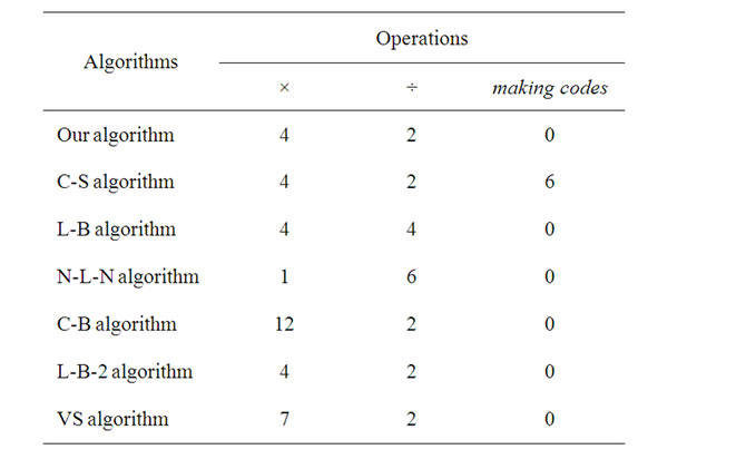
Table 1. The calculation complexities.
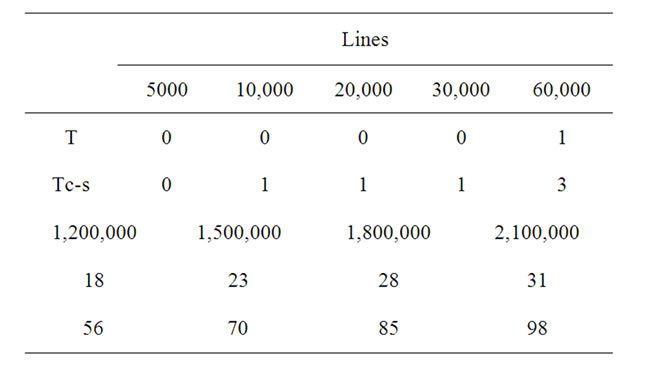
Table 2. The times of the clipping.
3) L-B-2 algorithm is 2.5 (the average) or 3.03 (the maximum) times [8] as fast as Cohen-Sutherland algorithm for the speed of line clipping.
4) The algorithm in this paper is 3.1 (the average) or 3.5 (the maximum) times as fast as Cohen-Sutherland algorithm, see Table 2.
From the facts above, we derive the conclusion that the algorithm in this paper is faster than the other algorithms in table 1 for line clipping.
7. Conclusions
For the special situation that the line segment or its extension (like the line segment d in Figure 1) intersects all the edges or their extensions of the window, the clipping speed of our algorithm is obviously faster than other algorithms. But for the random situations, the average clipping speed of our algorithm is a little bit faster than other algorithms.
8. References
[1] D. Hearn and M. P. Baker, “Computer Graphics,” C Version, 2nd Edition, Prentice Hall, Inc., Upper Saddle River, 1998, p. 226.
[2] M. Cyrus and J. Beck, “Generalized Two and Three Dimensional Clipping,” Computers and Graphics, Vol. 3, No. 1, 1978, pp. 23-28.
[3] D. Hearn and M. P. Baker, “Computer Graphics,” C Version, 2nd Edition, Prentice Hall, Inc., Upper Saddle River, 1998, p. 233.
[4] T. M. Nicholl, D. T. Lee and R. A. Nicholl, “An Efficient New Algorithm for 2-D Line Clipping: Its Development and Analysis,” Computers and Graphics, Vol. 21, No. 4, 1987, pp. 253-262.
[5] D. Hearn and M. P. Baker, “Computer Graphics,” C Version, 2nd Edition, Prentice Hall, Inc., Upper Saddle River, 1998, p. 230.
[6] C. B. Chen and F. Lu, “Computer Graphics Basis,” Publishing House of Electronics Industry, Beijing, 2006, pp. 167-168.
[7] V. Skala, “O (lg N) Line clipping Algorithm in E2,” Computers and Graphics, Vol. 18, No. 4, 1994, pp. 517- 527.
[8] Y. D. Liang and B. A. Barsky, “The Optimal Tree Algorithm for Line Clipping,” Technical Paper Distributed at Eurographics’92 Conference, Cambridge, 1992, pp. 1-38.
[9] V. Skala, “A New Approach to Line and Line Segment Clipping in Homogeneous Coordinates,” Visual Computer, Vol. 21, No. 11, 2005, pp. 905-914.
[10] Y. D. Liang, B. A. Barsky and M. Slater, “Some Improvements to a Parametric Line Clipping Algorithm,” Technical Report No. UCB/CSD 92/688, Computer Science Division, University of California, Berkeley, 1992, pp. 1-22.